5 Tips for a Smooth SSIS Upgrade to SQL Server 2012


5 Tips for a Smooth SSIS Upgrade to SQL Server 2012

SQL Server Technical Article


Writers: Runying Mao, Carla Sabotta

Technical Reviewers: David Noor, Jeanne Baker


Published: November 2011

Applies to: SQL Server 2012


Summary:
Microsoft SQL Server 2012 Integration Services (SSIS) provides significant improvements in both the developer and administration experience. This article provides tips that can help to make the upgrade to Microsoft SQL Server 2012 Integration Services successful. The tips address editing package configurations and specifically connection strings, converting configurations to parameters, converting packages to the project deployment model, updating Execute Package tasks to use project references and parameterizing the PackageName property.


Copyright


This document is provided “as-is”. Information and views expressed in this document, including URL and other Internet Web site references, may change without notice. You bear the risk of using it.

Some examples depicted herein are provided for illustration only and are fictitious.  No real association or connection is intended or should be inferred.

This document does not provide you with any legal rights to any intellectual property in any Microsoft product. You may copy and use this document for your internal, reference purposes.

© 2011 Microsoft. All rights reserved.


Contents

    1

Introduction    4

TIP #1: Edit Package Configuration and Data Source after upgrading    4

TIP #2: Convert to project deployment model using Project Conversion Wizard    6

TIP #3: Update Execute Package Task to use project reference and use parameter to pass data from parent package to child package    7

TIP #4: Parameterize PackageName property of Execute Package Task to dynamically configure which child package to run at execution time    9

TIP #5: Convert package configuration to parameter when possible    10

Conclusion    10


Introduction

Microsoft SQL Server 2012 Integration Services (SSIS) provides significant improvements in both the developer and administration experience. New SSIS features have been introduced in order to improve developer productivity, and simplify the deployment, configuration, management and troubleshooting of SSIS packages.

SQL Server 2012 Integration Services introduces the project as a self-contained, deployment unit. Common values can be shared among packages in the same project through project parameters and project connection managers. ETL developers can easily reference child packages that are inside the project.

Solutions that were created in earlier versions of SSIS (pre-SQL Server 2012) will be supported in SQL Server 2012. When you upgrade the solutions, you can take advantage of the new SQL Server 2012 features. Although in SQL Server 2012 SSIS offers wizards for upgrading most solution components, there will be a few settings that you’ll need to change manually.

Here are a few tips that can help to make the upgrade successful.

TIP #1: Edit Package Configuration and Data Source after upgrading


The first step to upgrade an SSIS solution is to run the SSIS Package Upgrade Wizard. The SSIS Package Upgrade Wizard makes appropriate changes to package properties and upgrades the package format.

The wizard launches when you open a pre-SQL Server 2012 package in the SQL Server Data Tools for the first time. SQL Server Data Tools replaces (BIDs). The wizard can also be launched manually by running SSISUpgrade.exe, which is located under %ProgramFiles%\Microsoft SQL Server\110\DTS\Binn.

It is critical to note that the SSIS Package Upgrade Wizard does not upgrade settings such as connection strings that are defined in the package configurations. After a package upgrade, you may need to make some manual changes to the package configuration to run the upgraded package successfully.

For example, you have an SSIS 2005 package. The package uses an OLE DB connection manager to connect to the AdventureWorks database in a local SQL Server 2005 instance. The package also uses an XML package configuration file to dynamically configure the ConnectionString property of the OLE DB connection manager. The following shows the contents of the XML package configuration file.

You have set up a machine with a standalone SQL Server 2012 installation. You move the SSIS 2005 package to the machine and run the SSIS Package Upgrade Wizard to upgrade the package to SQL Server 2012. When the wizard finishes, you need to manually change the provider name from SQLNCLI.1 to SQLNCLI11.1 in the XML package configuration file to run the upgraded package successfully. The wizard does not update package configuration files.

If you don’t update the provider name in the configuration file, the file configures the OLE DB connection manager to use the SQLNCLI.1 provider that is the SQL Server 2005 Native Client Library. SQLNCLI11.1 is the SQL Server 2012 Native Client Library. Because the SQL Server 2005 Native Client Library is not included in SQL Server 2012, the following error message will appear when you open or execute the upgraded package on the machine where SQL Server 2012 is installed:

The requested OLE DB provider SQLNCLI.1 is not registered. If the 32-bit driver is not installed, run the package in 64-bit mode. Error code: 0x00000000. An OLE DB record is available. Source: “Microsoft OLE DB Service Components” Hresult: 0x80040154 Description: “Class not registered”.

So, if your pre-SQL Server 2012 package uses any kind of package configurations, it is important to remember that you may need to manually update the content of the package configurations after you upgrade the package to SQL Server 2012. This applies to the different types of configurations, such as XML configuration files.

Connection strings that require updates and are stored in data source files or set by expressions, need to be updated manually.

TIP #2: Convert to project deployment model using Project Conversion Wizard


SQL Server 2012 SSIS supports two deployment models: the package deployment model and the project deployment model. The package deployment model was available in previous releases of SSIS and is the default deployment model for upgraded packages. In this model, the unit of deployment is the package. The project deployment model is new in SQL Server 2012 and provides additional package deployment and management features such as parameters and the Integration Services catalog. The unit of deployment is the project.

Please read Project Deployment Overview in SQL Server “Denali” CTP1 – SSIS (http://social.technet.microsoft.com/wiki/contents/articles/project-deployment-overview-in-sql-server-quot-denali-quot-ctp1-ssis.aspx ) for a detailed walk through as well as comparison between these two deployment models.

Read Projects in SQL Server “Denali” CTP1 – SSIS (http://social.technet.microsoft.com/wiki/contents/articles/projects-in-sql-server-denali-ctp1-ssis.aspx) for a thorough explanation of the new project concept.

To convert a package to the project deployment, right click the project in Solution Explorer and then click Convert to Project Deployment Model. The Project Conversion Wizard launches and walks you through the conversion process.

TIP #3: Update Execute Package Task to use project reference and use parameter to pass data from parent package to child package


If an SSIS package contains an Execute Package Task, the Project Conversion Wizard prompts you to update the task to use the project reference.

For example, your SSIS project contains several packages. Inside the project, one package (typically called the parent package) runs another package (typically called the child package) by using an Execute Package Task. In Pre-SQL Server 2012 releases of SSIS, the parent package references the child package by using a File connection manager. At deployment, you need to remember to update the File connection manager to ensure that it points to the new location of the child package.

In SQL Server 2012 Integration Services you can configure the parent package to reference the child package by name when the child package is included in the same project as the parent package. Using this project reference makes the deployment experience much smoother. You don’t need to remember to update the reference between the parent package and the child package at deployment. For a thorough explanation of the project reference in the Execute Package Task, please see Changes to the Execute Package Task (http://blogs.msdn.com/b/mattm/archive/2011/07/18/changes-to-the-execute-package-task.aspx).

In previous releases of SSIS, you pass data from the parent package to the child package by creating a package configuration that uses the parent variable configuration type. This enables a child package that is run from a parent package to access a variable in the parent.

It is recommended that you configure the Execute Package Task to use parameter binding to pass data from the parent package to the child package. Parameters make this task easier. For example, you want a parent package to dynamically determine the number of days in a current month and have the child package perform a task for that number of times. You can create a variable in the parent package that represents the number of days and create a parameter in the child package. Then in the Execute Package Task, you bind the parameter in the child package to the variable in the parent package.

Please read Parameters in SQL Server “Denali” CTP1 – SSIS (http://social.technet.microsoft.com/wiki/contents/articles/parameters-in-sql-server-denali-ctp1-ssis.aspx) for a description of parameters and the numerous benefits they offer.

TIP #4: Parameterize PackageName property of Execute Package Task to dynamically configure which child package to run at execution time


Suppose your SSIS 2008 package has an Execute Package Task, and the package uses a File connection manager to connect to a child package. You dynamically assign which child package the Execute Package Task runs by configuring the connection string property of the File connection manager.

The following is the content of the XML package configuration file used by your SSIS 2008 package.

When the Project Conversion Wizard converts the package to the project deployment model and updates the Execute Package Task to use the project reference, the File connection manager that was used to connect to the child package is no longer used by the Execute Package Task. To continue to dynamically determine which child package the task runs, you create a parameter and map that parameter to the PackageName property of the Execute Package Task as shown in the following image.

TIP #5: Convert package configuration to parameter when possible


Parameters are new to SQL Server 2012 Integration Services and are the replacement for package configurations. You use parameters to assign values to package properties, whether at design time or run time. The values are pushed to a package when it is executed rather than having the package pull values from the package configurations.

The Project Conversion Wizard prompts you to optionally convert package configurations to parameters. It is possible that you might choose to keep a package configuration as an intermediate step of upgrading to SQL Server 2012. When your package has both configuration values and parameter values, it is important to understand the order in which these values are applied. Package configuration values will be applied first. If there are also parameter values for the same properties, these values will be applied next and will overwrite the package configuration values.

Conclusion

Microsoft SQL Server 2012 Integration Services (SSIS) offers features that greatly enhance the development and administrative experience. These tips could help users ensure successful upgrades of their current solutions to SQL Server 2012 so that they can take advantage of SQL Server 2012’s new features. For more information about SQL Server 2012 Integration Services and what’s new, please refer to What’s New (Integration Services) (http://msdn.microsoft.com/en-us/library/bb522534(v=SQL.110).aspx).


Did this paper help you? Please give us your feedback. Tell us on a scale of 1 (poor) to 5 (excellent), how would you rate this paper and why have you given it this rating? For example:

  • Are you rating it high due to having good examples, excellent screen shots, clear writing, or another reason?
  • Are you rating it low due to poor examples, fuzzy screen shots, or unclear writing?

This feedback will help us improve the quality of white papers we release.

Send feedback.

SharePoint 2010 Best Practices

Intro

Best practices are, and rightfully so, always a much sought-after topic. There are various kinds of best practices:

  • Microsoft best practices. In real life, these are the most important ones to know, as most companies implementing SharePoint best practices have a tendency to follow as much of these as possibly can. Independent consultants doing architecture and code reviews will certainly take a look at these as well. In general, you can safely say that best practices endorsed by Microsoft have an added bonus and it will be mentioned whenever this is the case.
  • Best practices. These practices are patterns that have proven themselves over and over again as a way to achieve a high quality of your solutions, and it’s completely irrelevant who proposed them. Often MS best practices will also fall in this category. In real life, these practices should be the most important ones to follow.
  • Practices. These are just approaches that are reused over and over again, but not necessarily the best ones. Wiki’s are a great way to discern best practices from practices. It’s certainly possible that this page refers to these “Practices of the 3rd kind”, but hopefully, the SharePoint community will eventually filter them out. Therefore, everybody is invited and encouraged to actively participate in the various best practices discussions.

This Wiki page contains an overview of SharePoint 2010 Best Practices of all kinds, divided by categories.

Performance

When implementing IT solutions, everybody will face the day where a customer isn’t happy with the way an application is performing. Because of the complex infrastructure and vast amount of features of SharePoint, there are many ways to approach these issues. Because of that and the importance of the topic, our first category outlines best practices to tackling performance problems.

Planning

Every SharePoint undertaking will at one point face the following questions: how long will it take, how much will it cost to implement, and how will we use it?

Installation, Removal, Configuration, and Operation

This section deals with best practices regarding the following questions: How to install SharePoint? How to configure it? How to keep it operating? All best practices are targeted towards the IT Pro.

Deployment

Deployment of software artifacts is important. This section discusses best practices.

Virtualization

It’s very common that SharePoint farms use virtualization techniques. This section is dedicated to best practices concerning virtualization.

Real Life Usage

Once you have SharePoint deployed, it’s up to the end users, power users, and IT Pros to make the best of it. This section discusses best practices targeted towards this audience.

Backup and Recovery

This section deals with best practices about the back up and restore of SharePoint environments.

Development

This section covers best practices targeted towards software developers.

Search

Search is a complex topic and important to almost every company working with SharePoint. This section discusses best practices.

Upgrade and Migration

If a product is successful, it has to be upgraded at some point.

Extranet Environments

This section provides an overview of planning and design considerations for SharePoint Extranet Environments.

Farms

This section discusses best practices regarding SharePoint 2010 farm topologies.

Top 10 Blogs to Follow

It’s certainly a best practice to keep up to date with the latest SharePoint news. Therefore, a top 10 of blog suggestions to follow is included.

  1. http://blogs.msdn.com/b/sharepointdev/ , the SharePoint Developer team blog.
  2. http://www.andrewconnell.com/blog , Andrew Connell on SharePoint.
  3. http://www.sharepointjoel.com/default.aspx , Joel Oleson’s SharePoint Land.
  4. http://sharepointdragons.com , Nikander & Margriet on SharePoint.
  5. http://blogs.msdn.com/b/uksharepoint/ , the SharePoint guys.
  6. https://www.nothingbutsharepoint.com/Pages/default.aspx , Nothing but SharePoint.
  7. http://www.shillier.com/default.aspx , Scot Hillier on SharePoint.
  8. http://www.lightningtools.com/blog/default.aspx , Lightning Tools Blog.
  9. http://www.wictorwilen.se/ , Wictor Wilen on SharePoint.
  10. http://www.gokanozcifci.be/blog , Gokan Ozcifci on SharePoint

Top 5 SharePoint Books

Books remain the most important resource for learning a new topic. Here’s a suggestion of the best SharePoint 2010 books out there.

  1. http://www.amazon.com/Inside-Microsoft-SharePoint-2010-Pattison/dp/0735627460/ref=sr_1_1?s=books&ie=UTF8&qid=1337663232&sr=1-1 , the favorite developer book about SharePoint 2010.
  2. http://www.amazon.com/Microsoft-SharePoint-2010-Administrators-Companion/dp/0735627207/ref=sr_1_2?s=books&ie=UTF8&qid=1337603828&sr=1-2 , great resource for administrators.
  3. http://www.amazon.com/SharePoint-2010-Site-Owners-Manual/dp/1933988754/ref=sr_1_1?s=books&ie=UTF8&qid=1337663093&sr=1-1 , does a great job teaching SharePoint end users and power users.
  4. http://www.amazon.com/Microsoft-SharePoint-Designer-2010-Step/dp/0735627339/ref=sr_1_2?s=books&ie=UTF8&qid=1337663155&sr=1-2 , dedicated to SharePoint Designer 2010.
  5. http://www.amazon.com/SharePoint-2010-Web-Parts-Action/dp/1935182773/ref=sr_1_1?s=books&ie=UTF8&qid=1337663192&sr=1-1 , best book out there about SharePoint 2010 web parts.

Top 10 SharePoint Tools

What to put in your bag of tools?

  1. http://cksdev.codeplex.com/ , CKSDev makes SharePoint development easier.
  2. http://spm.codeplex.com/ , SharePoint Manager is a SharePoint object model explorer.
  3. http://camldotnet.codeplex.com/ , CAML.NET:  IntelliSense for CAML.
  4. http://karinebosch.wordpress.com/2012/05/12/caml-designer/ , CAML Designer makes creating CAML queries a lot easier (successor of U2U CAML Query Builder).
  5. http://archive.msdn.microsoft.com/ULSViewer , you’ll always need a tool to view the ULS log files. ULS Log Viewer is probably the most popular one of the lot.
  6. http://gallery.technet.microsoft.com/Maxer-for-SharePoint-2010-8cd0f26f , the SharePoint Maxer tool helps checking for capacity planning limits.
  7. http://gallery.technet.microsoft.com/The-SharePoint-Flavored-5b03f323 , the SharePoint Flavored Weblog Reader (SFWR) helps troubleshooting performance problems by analyzing the IIS log files of SharePoint WFEs.
  8. http://gallery.technet.microsoft.com/The-Migration-Dragon-for-628acae0 , the Migration Dragon for SharePoint 2010 is a tool that can help to migrate file and folder structures from the file system to SharePoint 2010 Document Libraries leveraging the batching mechanism of the SharePoint managed client object model.
  9. http://visualstudiogallery.msdn.microsoft.com/36a6eb45-a7b1-47c3-9e85-09f0aef6e879 , Muse.VSExtensions, a great tool for referencing assemblies located in the GAC.
  10. http://spservices.codeplex.com/ , jQuery Library for SharePoint Web Services

Top Forums/Communities

Here is a list of sites to ask questions.

  1. Sharepoint StackExchange
  2. Microsoft SharePoint Products and Technologies Forum

Microsoft SQL Server 2005 Analysis Services Performance Guide


Microsoft SQL Server 2005 Analysis Services Performance Guide

SQL Server Technical Article


Author:     Elizabeth Vitt


Subject Matter Experts:

T.K. Anand

Sasha (Alexander) Berger

Marius Dumitru

Eric Jacobsen

Edward Melomed

Akshai Mirchandani

Mosha Pasumansky

Cristian Petculescu

Carl Rabeler

Wayne Robertson

Richard Tkachuk

Dave Wickert

Len Wyatt


Published: February 2007

Applies To: SQL Server 2005, Service Pack 2


Summary: This white paper describes how application developers can apply performance-tuning techniques to their Microsoft SQL Server 2005 Analysis Services Online Analytical Processing (OLAP) solutions.


The information contained in this document represents the current view of Microsoft Corporation on the issues discussed as of the date of publication. Because Microsoft must respond to changing market conditions, it should not be interpreted to be a commitment on the part of Microsoft, and Microsoft cannot guarantee the accuracy of any information presented after the date of publication.


This White Paper is for informational purposes only. MICROSOFT MAKES NO WARRANTIES, EXPRESS, IMPLIED OR STATUTORY, AS TO THE INFORMATION IN THIS DOCUMENT.


Complying with all applicable copyright laws is the responsibility of the user. Without limiting the rights under copyright, no part of this document may be reproduced, stored in or introduced into a retrieval system, or transmitted in any form or by any means (electronic, mechanical, photocopying, recording, or otherwise), or for any purpose, without the express written permission of Microsoft Corporation.


Microsoft may have patents, patent applications, trademarks, copyrights, or other intellectual property rights covering subject matter in this document. Except as expressly provided in any written license agreement from Microsoft, the furnishing of this document does not give you any license to these patents, trademarks, copyrights, or other intellectual property.


Unless otherwise noted, the companies, organizations, products, domain names, e-mail addresses, logos, people, places, and events depicted in examples herein are fictitious. No association with any real company, organization, product, domain name, e-mail address, logo, person, place, or event is intended or should be inferred.


2007 Microsoft Corporation. All rights reserved.


Microsoft, Windows, and Windows Server
are either registered trademarks or trademarks of Microsoft Corporation in the United States and/or other countries.


All other trademarks are property of their respective owners.


Table of Contents

Introduction    6

Enhancing Query Performance    8

Understanding the querying architecture    8

Session management    9

MDX query execution    10

Data retrieval: dimensions    12

Data retrieval: measure group data    15

Optimizing the dimension design    18

Identifying attribute relationships    18

Using hierarchies effectively    22

Maximizing the value of aggregations    24

How aggregations help    24

How the Storage Engine uses aggregations    25

Why not create every possible aggregation?    27

How to interpret aggregations    29

Which aggregations are built    30

How to impact aggregation design    31

Suggesting aggregation candidates    32

Specifying statistics about cube data    36

Adopting an aggregation design strategy    39

Using partitions to enhance query performance    40

How partitions are used in querying    41

Designing partitions    41

Aggregation considerations for multiple partitions    43

Writing efficient MDX    44

Specifying the calculation space    44

Removing empty tuples    47

Summarizing data with MDX    55

Taking advantage of the Query Execution Engine cache    58

Applying calculation best practices    60

Tuning Processing Performance    61

Understanding the processing architecture    61

Processing job overview    61

Dimension processing jobs    62

Dimension-processing commands    64

Partition-processing jobs    65

Partition-processing commands    65

Executing processing jobs    66

Refreshing dimensions efficiently    67

Optimizing the source query    67

Reducing attribute overhead    68

Optimizing dimension inserts, updates, and deletes    70

Refreshing partitions efficiently    71

Optimizing the source query    71

Using partitions to enhance processing performance    72

Optimizing data inserts, updates, and deletes    72

Evaluating rigid vs. flexible aggregations    73

Optimizing Special Design Scenarios    76

Special aggregate functions    76

Optimizing distinct count    76

Optimizing semiadditive measures    78

Parent-child hierarchies    79

Complex dimension relationships    79

Many-to-many relationships    80

Reference relationships    82

Near real-time data refreshes    86

Tuning Server Resources    91

Understanding how Analysis Services uses memory    92

Memory management    92

Shrinkable vs. non-shrinkable memory    94

Memory demands during querying    95

Memory demands during processing    96

Optimizing memory usage    97

Increasing available memory    97

Monitoring memory management    97

Minimizing metadata overhead    98

Monitoring the timeout of idle sessions    99

Tuning memory for partition processing    100

Warming the data cache    101

Understanding how Analysis Services uses CPU resources    103

Job architecture    103

Thread pools    103

Processor demands during querying    104

Processor demands during processing    104

Optimizing CPU usage    105

Maximize parallelism during querying    105

Maximize parallelism during processing    107

Use sufficient memory    109

Use a load-balancing cluster    109

Understanding how Analysis Services uses disk resources    110

Disk resource demands during processing    110

Disk resource demands during querying    110

Optimizing disk usage    111

Using sufficient memory    111

Optimizing file locations    111

Disabling unnecessary logging    111

Conclusion    112

Appendix A – For More Information    113

Appendix B – Partition Storage Modes    113

Multidimensional OLAP (MOLAP)    113

Hybrid OLAP (HOLAP)    114

Relational OLAP (ROLAP)    115

Appendix C – Aggregation Utility    116

Benefits of the Aggregation Utility    116

How the Aggregation Utility organizes partitions    117

How the Aggregation Utility works    118


Introduction

Fast query response times and timely data refresh are two well-established performance requirements of Online Analytical Processing (OLAP) systems. To provide fast analysis, OLAP systems traditionally use hierarchies to efficiently organize and summarize data. While these hierarchies provide structure and efficiency to analysis, they tend to restrict the analytic freedom of end users who want to freely analyze and organize data on the fly.

To support a broad range of structured and flexible analysis options, Microsoft® SQL Server™ Analysis Services (SSAS) 2005 combines the benefits of traditional hierarchical analysis with the flexibility of a new generation of attribute hierarchies. Attribute hierarchies allow users to freely organize data at query time, rather than being limited to the predefined navigation paths of the OLAP architect. To support this flexibility, the Analysis Services OLAP architecture is specifically designed to accommodate both attribute and hierarchical analysis while maintaining the fast query performance of conventional OLAP databases.

Realizing the performance benefits of this combined analysis paradigm requires understanding how the OLAP architecture supports both attribute hierarchies and traditional hierarchies, how you can effectively use the architecture to satisfy your analysis requirements, and how you can maximize the architecture’s utilization of system resources.

Note   To apply the performance tuning techniques discussed in this white paper, you must have SQL Server 2005 Service Pack 2 installed.

To satisfy the performance needs of various OLAP designs and server environments, this white paper provides extensive guidance on how you can take advantage of the wide range of opportunities to optimize Analysis Services performance. Since Analysis Services performance tuning is a fairly broad subject, this white paper organizes performance tuning techniques into the following four segments.

Enhancing Query Performance – Query performance directly impacts the quality of the end user experience. As such, it is the primary benchmark used to evaluate the success of an OLAP implementation. Analysis Services provides a variety of mechanisms to accelerate query performance, including aggregations, caching, and indexed data retrieval. In addition, you can improve query performance by optimizing the design of your dimension attributes, cubes, and MDX queries.

Tuning Processing Performance – Processing is the operation that refreshes data in an Analysis Services database. The faster the processing performance, the sooner users can access refreshed data. Analysis Services provides a variety of mechanisms that you can use to influence processing performance, including efficient dimension design, effective aggregations, partitions, and an economical processing strategy (for example, incremental vs. full refresh vs. proactive caching).

Optimizing Special Design Scenarios
– Complex design scenarios require a distinct set of performance tuning techniques to ensure that they are applied successfully, especially if you combine a complex design with large data volumes. Examples of complex design components include special aggregate functions, parent-child hierarchies, complex dimension relationships, and “near real-time” data refreshes.

Tuning Server Resources

Analysis Services operates within the constraints of available server resources. Understanding how Analysis Services uses memory, CPU, and disk resources can help you make effective server management decisions that optimize querying and processing performance.

Three appendices provide links to additional resources, information on various partition storage modes, and guidance on using the Aggregation Utility that is a part of SQL Server 2005 Service Pack 2 samples.


Enhancing Query Performance

Querying is the operation where Analysis Services provides data to client applications according to the calculation and data requirements of a MultiDimensional eXpressions (MDX) query. Since query performance directly impacts the user experience, this section describes the most significant opportunities to improve query performance. Following is an overview of the query performance topics that are addressed in this section:

Understanding the querying architecture – The
Analysis Services querying architecture supports three major operations: session management, MDX query execution, and data retrieval. Optimizing query performance involves understanding how these three operations work together to satisfy query requests.

Optimizing the dimension design – A well-tuned dimension design is perhaps one of the most critical success factors of a high-performing Analysis Services solution. Creating attribute relationships and exposing attributes in hierarchies are design choices that influence effective aggregation design, optimized MDX calculation resolution, and efficient dimension data storage and retrieval from disk.

Maximizing the value of aggregations – Aggregations improve query performance by providing precalculated summaries of data. To maximize the value of aggregations, ensure that you have an effective aggregation design that satisfies the needs of your specific workload.

Using partitions to enhance query performance – Partitions provide a mechanism to separate measure group data into physical units that improve query performance, improve processing performance, and facilitate data management. Partitions are naturally queried in parallel; however, there are some design choices and server property optimizations that you can specify to optimize partition operations for your server configuration.

Writing efficient MDX – This section describes techniques for writing efficient MDX statements such as: 1) writing statements that address a narrowly defined calculation space, 2) designing calculations for the greatest re-usage across multiple users, and 3) writing calculations in a straight-forward manner to help the Query Execution Engine select the most efficient execution path.

Understanding the querying architecture

To make the querying experience as fast as possible for end users, the Analysis Services querying architecture provides several components that work together to efficiently retrieve and evaluate data. Figure 1 identifies the three major operations that occur during querying: session management, MDX query execution, and data retrieval as well as the server components that participate in each operation.


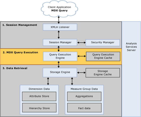
Figure 1   Analysis Services querying architecture

Session management

Client applications communicate with Analysis Services using XML for Analysis (XMLA) over TCP IP or HTTP. Analysis Services provides an XMLA listener component that handles all XMLA communications between Analysis Services and its clients. The Analysis Services Session Manager controls how clients connect to an Analysis Services instance. Users authenticated by Microsoft® Windows and who have rights to Analysis Services can connect to Analysis Services. After a user connects to Analysis Services, the Security Manager determines user permissions based on the combination of Analysis Services roles that apply to the user. Depending on the client application architecture and the security privileges of the connection, the client creates a session when the application starts, and then reuses the session for all of the user’s requests. The session provides the context under which client queries are executed by the Query Execution Engine. A session exists until it is either closed by the client application, or until the server needs to expire it. For more information regarding the longevity of sessions, see Monitoring the timeout of idle sessions in this white paper.

MDX query execution

The primary operation of the Query Execution Engine is to execute MDX queries. This section provides an overview of how the Query Execution Engine executes queries. To learn more details about optimizing MDX, see Writing efficient MDX later in this white paper.

While the actual query execution process is performed in several stages, from a performance perspective, the Query Execution engine must consider two basic requirements: retrieving data and producing the result set.

  1. Retrieving data—To retrieve the data requested by a query, the Query Execution Engine decomposes each MDX query into data requests. To communicate with the Storage Engine, the Query Execution Engine must translate the data requests into subcube requests that the Storage Engine can understand. A subcube represents a logical unit of querying, caching, and data retrieval. An MDX query may be resolved into one or more subcube requests depending on query granularity and calculation complexity. Note that the word subcube is a generic term. For example, the subcubes that the Query Execution Engine creates during query evaluation are not to be confused with the subcubes that you can create using the MDX CREATE SUBCUBE statement.
  2. Producing the result set—To manipulate the data retrieved from the Storage Engine, the Query Execution Engine uses two kinds of execution plans to calculate results: it can bulk calculate an entire subcube, or it can calculate individual cells. In general, the subcube evaluation path is more efficient; however, the Query Execution Engine ultimately selects execution plans based on the complexities of each MDX query. Note that a given query can have multiple execution plans for different parts of the query and/or different calculations involved in the same query. Moreover, different parts of a query may choose either one of these two types of execution plans independently, so there is not a single global decision for the entire query. For example, if a query requests resellers whose year-over-year profitability is greater than 10%, the Query Execution Engine may use one execution plan to calculate each reseller’s year-over-year profitability and another execution plan to only return those resellers whose profitability is greater than 10%.

    When you execute an MDX calculation, the Query Execution Engine must often execute the calculation across more cells than you may realize. Consider the example where you have an MDX query that must return the calculated year-to-date sales across the top five regions. While it may seem like you are only returning five cell values, Analysis Services must execute the calculation across additional cells in order to determine the top five regions and also to return their year to date sales. A general MDX optimization technique is to write MDX queries in a way that minimizes the amount of data that the Query Execution Engine must evaluate. To learn more about this MDX optimization technique, see Specifying the calculation space later in this white paper.

    As the Query Execution Engine evaluates cells, it uses the Query Execution Engine cache and the Storage Engine Cache to store calculation results. The primary benefits of the cache are to optimize the evaluation of calculations and to support the re-usage of calculation results across users. To optimize cache re-usage, the Query Execution Engine manages three cache scopes that determine the level of cache reusability: global scope, session scope, and query scope. For more information on cache sharing, see Taking advantage of the Query Execution Engine cache in this white paper.


Data retrieval: dimensions

During data retrieval, the Storage Engine must efficiently choose the best mechanism to fulfill the data requests for both dimension data and measure data.

To satisfy requests for dimension data, the Storage Engine extracts data from the dimension attribute and hierarchy stores. As it retrieves the necessary data, the Storage Engine uses dynamic on-demand caching of dimension data rather than keeping all dimension members statically mapped into memory. The Storage Engine simply brings members into memory as they are needed. Dimension data structures may reside on disk, in Analysis Services memory, or in the Windows operating system file cache, depending on memory load of the system.

As the name suggests, the Dimension Attribute Store contains all of the information about dimension attributes. The components of the Dimension Attribute Store are displayed in Figure 2.


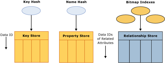
Figure 2   Dimension Attribute Store

As displayed in the diagram, the Dimension Attribute Store contains the following components for each attribute in the dimension:

  • Key store—The key store contains the attribute’s key member values as well as an internal unique identifier called a DataID. Analysis Services assigns the DataID to each attribute member and uses the same DataID to refer to that member across all of its stores.
  • Property store—The property store contains a variety of attribute properties, including member names and translations. These properties map to specific DataIDs. DataIDs are contiguously allocated starting from zero. Property stores as well as relationship stores (relationship stores are discussed in more detail later) are physically ordered by DataID, in order to ensure fast random access to the contents, without additional index or hash table lookups.
  • Hash tables—To facilitate attribute lookups during querying and processing, each attribute has two hash tables which are created during processing and persisted on disk. The Key Hash Table indexes members by their unique keys. A Name Hash Table indexes members by name.
  • Relationship store—The Relationship store contains an attribute’s relationships to other attributes. More specifically, the Relationship store stores each source record with DataID references to other attributes. Consider the following example for a product dimension. Product is the key attribute of the dimension with direct attribute relationships to color and size. The data instance of product Sport Helmet, color of Black, and size of Large may be stored in the relationship store as 1001, 25, 5 where 1001 is the DataID for Sport Helmet, 25 is the Data ID for Black, and 5 is the Data ID for Large. Note that if an attribute has no attribute relationships to other attributes, a Relationship Store is not created for that particular attribute. For more information on attribute relationships, see Identifying attribute relationships in this whitepaper.
  • Bitmap indexes—To efficiently locate attribute data in the Relationship Store at querying time, the Storage Engine creates bitmap indexes at processing time. For each DataID of a related attribute, the bitmap index states whether or not a page contains at least one record with that DataID. For attributes with a very large number of DataIDs, the bitmap indexes can take some time to process. In most scenarios, the bitmap indexes provide significant querying benefits; however, there is a design scenario where the querying benefit that the bitmap index provides does not outweigh the processing cost of creating the bitmap index in the first place. It is possible to remove the bitmap index creation for a given attribute by setting the AttributeHierarchyOptimizedState property to Not Optimized. For more information on this design scenario, see Reducing attribute overhead in this white paper.

In addition to the attribute store, the Hierarchy Store arranges attributes into navigation paths for end users as displayed in Figure 3.


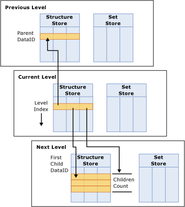
Figure 3   Hierarchy stores

The Hierarchy store consists of the following primary components:

  • Set StoreThe Set Store uses DataIDs to construct the path of each member, mapped from the first level to the current level. For example, All, Bikes, Mountain Bikes, Mountain Bike 500 may be represented as 1,2,5,6 where 1 is the DataID for All, 2 is the DataID for Bikes, 5 is the DataID for Mountain Bikes, and 6 is the DataID for Mountain Bike 500.
  • Structure StoreFor each member in a level, the Structure Store contains the DataID of the parent member, the DataID of the first child, and the total children count. The entries in the Structure Store are ordered by each member’s Level index. The Level index of a member is the position of a member in the level as specified by the ordering settings of the dimension. To better understand the Structure Store, consider the following example. If Bikes contains 3 children, the entry for Bikes in the Structure Store would be 1,5,3 where 1 is the DataID for the Bike’s parent, All, 5 is the DataID for Mountain Bikes, and 3 is the number of Bike’s children.

Note that only natural hierarchies are materialized in the hierarchy store and optimized for data retrieval. Unnatural hierarchies are not materialized on disk. For more information on the best practices for designing hierarchies, see Using hierarchies effectively.

Data retrieval: measure group data

For data requests, the Storage Engine retrieves measure group data that is physically stored in partitions. A partition contains two categories of measure group data: fact data and aggregations. To accommodate a variety of data storage architectures, each partition can be assigned a different storage mode that specifies where fact data and aggregations are stored. From a performance perspective, the storage mode that provides the fastest query performance is the Multidimensional Online Analytical Processing (MOLAP) storage mode. In MOLAP, the partition fact data and aggregations are stored in a compressed multidimensional format that Analysis Services manages. For most implementations, MOLAP storage mode should be used; however, if you require additional information about other partition storage modes, see Appendix B. If you are considering a “near real-time” deployment, see Near real-time data refreshes in this white paper.

In MOLAP storage, the data structures for fact data and aggregation data are identical. Each is divided into segments. A segment contains a fixed number of records (typically 64 KB) divided into 256 pages with 256 records in each. Each record stores all of the measures in the partition’s measure group and a set of internal DataIDs that map to the granularity attributes of each dimension. Only records that are present in the relational fact table are stored in the partition, resulting in highly compressed data files.

To efficiently fulfill data requests, the Storage Engine follows an optimized process to satisfy the request by using three general mechanisms, Storage Engine Cache, aggregations, and fact data represented in Figure 4:.


Figure 4   Satisfying data requests

Figure 4 presents a data request for {(Europe, 2005), (Asia, 2005)}. To fulfill this request, the Storage Engine chooses among the following approaches:

  • Storage Engine cache—The Storage Engine first attempts to satisfy the data request using the Storage Engine cache. Servicing a data request from the Storage Engine cache provides the best query performance. The Storage Engine cache always resides in memory. For more information on managing the Storage Engine cache, see Memory demands during querying.
  • Aggregations—If relevant data is not in the cache, the Storage Engine checks for a precalculated data aggregation. In some scenarios, the aggregation may exactly fit the data request. For example, an exact fit occurs when the query asks for sales by category by year and there is an aggregation that summarizes sales by category by year. While an exact fit is ideal, the Storage Engine can use also data aggregated at a lower level, such as sales aggregated by month and category or sales aggregated by quarter and item. The Storage Engine then summarizes the values on the fly to produce sales by category by year. For more information on how to design aggregations to improve performance, see Maximizing the value of aggregations.
  • Fact data—If appropriate aggregations do not exist for a given query, the Storage Engine must retrieve the fact data from the partition. The Storage Engine uses many internal optimizations to effectively retrieve data from disk including enhanced indexing and clustering of related records. For both aggregations and fact data, different portions of data may reside either on disk or in the Windows operating system file cache, depending on memory load of the system.

A key performance tuning technique for optimizing data retrieval is to reduce the amount of data that the Storage Engine needs to scan by using multiple partitions that physically divide your measure group data into distinct data slices. Using multiple partitions can not only enhance querying speed, but they can also provide greater scalability, facilitate data management, and optimize processing performance.

From a querying perspective, the Storage Engine can predetermine the data stored in each MOLAP partition and optimize which MOLAP partitions it scans in parallel. In the example in Figure 4, a partition with 2005 data is displayed in blue and a partition with 2006 data is displayed in orange. The data request displayed in the diagram {(Europe, 2005), (Asia, 2005)} only requires 2005 data. Consequently, the Storage Engine only needs to go to the 2005 partition. To maximize query performance, the Storage Engine uses parallelism, such as scanning partitions in parallel, wherever possible. To locate data in a partition, the Storage Engine queries segments in parallel and uses bitmap indexes to efficiently scan pages to find the desired data.

Partitions are a major component of high-performing cubes. For more information on the broader benefits of partitions, see the following sections in this white paper:


Optimizing the dimension design

A well-tuned dimension design is one of the most critical success factors of a high-performing Analysis Services solution. The two most important techniques that you can use to optimize your dimension design for query performance are:

  • Identifying attribute relationships
  • Using hierarchies effectively
Identifying attribute relationships

A typical data source of an Analysis Services dimension is a relational data warehouse dimension table. In relational data warehouses, each dimension table typically contains a primary key, attributes, and, in some cases, foreign key relationships to other tables.

Table 1   Column properties of a simple Product dimension table

Dimension table column

Column type

Relationship to primary key

Relationship to other columns

Product Key

Primary Key 

Primary Key 

Product SKU  

Attribute 

1:1 

Description 

Attribute 

1:1 

Color 

Attribute 

Many:1 

Size  

Attribute 

Many:1 

Many: 1 to Size Range

Size Range 

Attribute 

Many:1 


Subcategory 

Attribute 

Many:1 

Many: 1 to Category

Category

Attribute 

Many:1 


Table 1 displays the design of a simple product dimension table. In this simple example, the product dimension table has one primary key column, the product key. The other columns in the dimension table are attributes that provide descriptive context to the primary key such as product SKU, description, and color. From a relational perspective, all of these attributes either have a many-to-one relationship to the primary key or a one-to-one relationship to the primary key. Some of these attributes also have relationships to other attributes. For example, size has a many-to-one relationship with size range and subcategory has a many-to-one relationship with category.

Just as it is necessary to understand and define the functional dependencies among fields in relational databases, you must also follow the same practices in Analysis Services. Analysis Services must understand the relationships among your attributes in order to correctly aggregate data, effectively store and retrieve data, and create useful aggregations. To help you create these associations among your dimension attributes, Analysis Services provides a feature called attribute relationships. As the name suggests, an attribute relationship describes the relationship between two attributes.

When you initially create a dimension, Analysis Services auto-builds a dimension structure with many-to-one attribute relationships between the primary key attribute and every other dimension attribute as displayed in Figure 5.


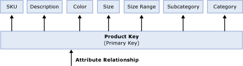
Figure 5   Default attribute relationships

The arrows in Figure 5 represent the attribute relationships between product key and the other attributes in the dimension. While the dimension structure presented in Figure 5 provides a valid representation of the data from the product dimension table, from a performance perspective, it is not an optimized dimension structure since Analysis Services is not aware of the relationships among the attributes.

With this design, whenever you issue a query that includes an attribute from this dimension, data is always summarized from the primary key and then grouped by the attribute. So if you want sales summarized by Subcategory, individual product keys are grouped on the fly by Subcategory. If your query requires sales by Category, individual product keys are once again grouped on the fly by Category. This is somewhat inefficient since Category totals could be derived from Subcategory totals. In addition, with this design, Analysis Services doesn’t know which attribute combinations naturally exist in the dimension and must use the fact data to identify meaningful member combinations. For example, at query time, if a user requests data by Subcategory and Category, Analysis Services must do extra work to determine that the combination of Subcategory: Mountain Bikes and Category: Accessories does not exist.

To optimize this dimension design, you must understand how your attributes are related to each other and then take steps to let Analysis Services know what the relationships are.

To enhance the product dimension, the structure in Figure 6 presents an optimized design that more effectively represents the relationships in the dimension.


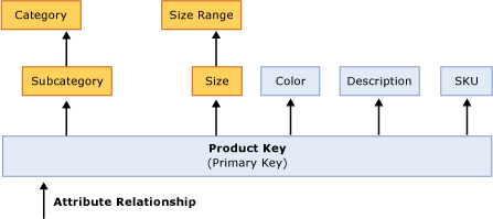
Figure 6   Product dimension with optimized attribute relationships

Note that the dimension design in Figure 6 is different than the design in Figure 5. In Figure 5, the primary key has attribute relationships to every other attribute in the dimension. In Figure 6, two new attribute relationships have been added between Size and Size Range and Subcategory and Category.

The new relationships between Size and Size Range and Subcategory and Category reflect the many-to-one relationships among the attributes in the dimension. Subcategory has a many-to-one relationship with Category. Size has a many-to-one relationship to Size Range. These new relationships tell Analysis Services how the nonprimary key attributes (Size and Size Range, and Subcategory and Category) are related to each other.

Typically many-to-one relationships follow data hierarchies such as the hierarchy of products, subcategories, and categories depicted in Figure 6. While a data hierarchy can commonly suggest many-to-one relationships, do not automatically assume that this is always the case. Whenever you add an attribute relationship between two attributes, it is important to first verify that the attribute data strictly adheres to a many-to-one relationship. As a general rule, you should create an attribute relationship from attribute A to attribute B if and only if the number of distinct (a, b) pairs from A and B is the same (or smaller) than the number of distinct members of A. If you create an attribute relationship and the data violates the many-to-one relationship, you will receive incorrect data results.

Consider the following example. You have a time dimension with a month attribute containing values such as January, February, March and a year attribute containing values such as 2004, 2005, and 2006. If you define an attribute relationship between the month and year attributes, when the dimension is processed, Analysis Services does not know how to distinguish among the months for each year. For example, when it comes across the January member, it does not which year should it roll it up to. The only way to ensure that data is correctly rolled up from month to year is to change the definition of the month attribute to month and year. You make this definition change by changing the KeyColumns property of the attribute to be a combination of month and year.

The KeyColumns property consists of a source column or combination of source columns (known as a collection) that uniquely identifies the members for a given attribute. Once you define attribute relationships among your attributes, the importance of the KeyColumns property is highlighted. For every attribute in your dimension, you must ensure that the KeyColumns property of each attribute uniquely identifies each attribute member. If the KeyColumns property does not uniquely identify each member, duplicates encountered during processing are ignored by default, resulting in incorrect data rollups.

Note that if the attribute relationship has a default Type of Flexible, Analysis Services does not provide any notification that it has encountered duplicate months and incorrectly assigns all of the months to the first year or last year depending on data refresh technique. For more information on the Type property and the impact of your data refresh technique on key duplicate handling, see Optimizing dimension inserts, updates, and deletes in this white paper.

Regardless of your data refresh technique, key duplicates typically result in incorrect data rollups and should be avoided by taking the time to set a unique KeyColumns property. Once you have correctly configured the KeyColumns property to uniquely define an attribute, it is a good practice to change the default error configuration for the dimension so that it no longer ignores duplicates. To do this, set the KeyDuplicate property from IgnoreError to ReportAndContinue or ReportAndStop. With this change, you can be alerted of any situation where the duplicates are detected.

Whenever you define a new attribute relationship, it is critical that you remove any redundant relationships for performance and data correctness. In Figure 6, with the new attribute relationships, the Product Key no longer requires direct relationships to Size Range or Category. As such, these two attribute relationships have been removed. To help you identify redundant attribute relationships, Business Intelligence Development Studio provides a visual warning to alert you about the redundancy; however, it does not require you to eliminate the redundancy. It is a best practice to always manually remove the redundant relationship. Once you remove the redundancy, the warning disappears.

Even though Product Key is no longer directly related to Size Range and Category, it is still indirectly related to these attributes through a chain of attribute relationships. More specifically, Product Key is related to Size Range using the chain of attribute relationships that link Product Key to Size and Size to Size Range. This chain of attribute relationships is also called cascading attribute relationships.

With cascading attribute relationships, Analysis Services can make better performance decisions concerning aggregation design, data storage, data retrieval, and MDX calculations. Beyond performance considerations, attribute relationships are also used to enforce dimension security and to join measure group data to nonprimary key granularity attributes. For example, if you have a measure group that contains sales data by Product Key and forecast data by Subcategory, the forecast measure group will only know how to roll up data from Subcategory to Category if attribute relationships exists between Subcategory and Category.

The core principle behind designing effective attribute relationships is to create the most efficient dimension model that best represents the semantics of your business. While this section provides guidelines and best practices for optimizing your dimension design, to be successful, you must be extremely familiar with your data and the business requirements that the data must support before considering how to tune your design.

Consider the following example. You have a time dimension with an attribute called Day of Week. This attribute contains seven members, one for each day of the week, where the Monday member represents all of the Mondays in your time dimension. Given what you learned from the month / year example, you may think that you should immediately change the KeyColumns property of this attribute to concatenate the day with the calendar date or some other attribute. However, before making this change, you should consider your business requirements. The day-of-week grouping can be valuable in some analysis scenarios such as analyzing retail sales patterns by the day of the week. However, in other applications, the day of the week may only be interesting if it is concatenated with the actual calendar date. In other words, the best design depends on your analysis scenario. So while it is important to follow best practices for modifying dimension properties and creating efficient attribute relationships, ultimately you must ensure that your own business requirements are satisfied. For additional thoughts on various dimension designs for a time dimension, see the blog Time calculations in UDM: Parallel Period.

Using hierarchies effectively

In Analysis Services, attributes can be exposed to users by using two types of hierarchies: attribute hierarchies and user hierarchies. Each of these hierarchies has a different impact on the query performance of your cube.

Attribute hierarchies are the default hierarchies that are created for each dimension attribute to support flexible analysis. For non parent-child hierarchies, each attribute hierarchy consists of two levels: the attribute itself and the All level. The All level is automatically exposed as the top level attribute of each attribute hierarchy.

Note that you can disable the All attribute for a particular attribute hierarchy by using the IsAggregatable property. Disabling the All attribute is generally not advised in most design scenarios. Without the All attribute, your queries must always slice on a specific value from the attribute hierarchy. While you can explicitly control the slice by using the Default Member property, realize that this slice applies across all queries regardless of whether your query specifically references the attribute hierarchy. With this in mind, it is never a good idea to disable the All attribute for multiple attribute hierarchies in the same dimension.

From a performance perspective, attributes that are only exposed in attribute hierarchies are not automatically considered for aggregation. This means that no aggregations include these attributes. Queries involving these attributes are satisfied by summarizing data from the primary key. Without the benefit of aggregations, query performance against these attributes hierarchies can be somewhat slow.

To enhance performance, it is possible to flag an attribute as an aggregation candidate by using the Aggregation Usage property. For more detailed information on this technique, see Suggesting aggregation candidates in this white paper. However, before you modify the Aggregation Usage property, you should consider whether you can take advantage of user hierarchies.

In user hierarchies, attributes are arranged into predefined multilevel navigation trees to facilitate end user analysis. Analysis Services enables you to build two types of user hierarchies: natural and unnatural hierarchies, each with different design and performance characteristics.

  • In a natural hierarchy, all attributes participating as levels in the hierarchy have direct or indirect attribute relationships from the bottom of the hierarchy to the top of the hierarchy. In most scenarios, natural hierarchies follow the chain of many-to-one relationships that “naturally” exist in your data. In the product dimension example discussed earlier in Figure 6, you may decide to create a Product Grouping hierarchy that from bottom-to-top consists of Products, Product Subcategories, and Product Categories. In this scenario, from the bottom of the hierarchy to the top of the hierarchy, each attribute is directly related to the attribute in the next level of the hierarchy. In an alternative design scenario, you may have a natural hierarchy that from bottom to top consists of Products and Product Categories. Even though Product Subcategories has been removed, this is still a natural hierarchy since Products is indirectly related to Product Category via cascading attribute relationships.
  • In an unnatural hierarchy the hierarchy consists of at least two consecutive levels that have no attribute relationships. Typically these hierarchies are used to create drill-down paths of commonly viewed attributes that do not follow any natural hierarchy. For example, users may want to view a hierarchy of Size Range and Category or vice versa.

From a performance perspective, natural hierarchies behave very differently than unnatural hierarchies. In natural hierarchies, the hierarchy tree is materialized on disk in hierarchy stores. In addition, all attributes participating in natural hierarchies are automatically considered to be aggregation candidates. This is a very important characteristic of natural hierarchies, important enough that you should consider creating natural hierarchies wherever possible. For more information on aggregation candidates, see Suggesting aggregation candidates.

Unnatural hierarchies are not materialized on disk and the attributes participating in unnatural hierarchies are not automatically considered as aggregation candidates. Rather, they simply provide users with easy-to-use drill-down paths for commonly viewed attributes that do not have natural relationships. By assembling these attributes into hierarchies, you can also use a variety of MDX navigation functions to easily perform calculations like percent of parent. An alternative to using unnatural hierarchies is to cross-join the data by using MDX at query time. The performance of the unnatural hierarchies vs. cross-joins at query time is relatively similar. Unnatural hierarchies simply provide the added benefit of reusability and central management.

To take advantage of natural hierarchies, you must make sure that you have correctly set up cascading attribute relationships for all attributes participating in the hierarchy. Since creating attribute relationships and creating hierarchies are two separate operations, it is not uncommon to inadvertently miss an attribute relationship at some point in the hierarchy. If a relationship is missing, Analysis Services classifies the hierarchy as an unnatural hierarchy, even if you intended it be a natural hierarchy.

To verify the type of hierarchy that you have created, Business Intelligence Development Studio issues a warning icon whenever you create a user hierarchy that is missing one or more attribute relationships. The purpose of the warning icon is to help identify situations where you have intended to create a natural hierarchy but have inadvertently missed attribute relationships. Once you create the appropriate attribute relationships for the hierarchy in question, the warning icon disappears. If you are intentionally creating an unnatural hierarchy, the hierarchy continues to display the warning icon to indicate the missing relationships. In this case, simply ignore the warning icon.

In addition, while this is not a performance issue, be mindful of how your attribute hierarchies, natural hierarchies, and unnatural hierarchies are displayed to end users in your front end tool. For example, if you have a series of geography attributes that are generally queried by using a natural hierarchy of Country/Region, State/Province, and City, you may consider hiding the individual attribute hierarchies for each of these attributes in order to prevent redundancy in the user experience. To hide the attribute hierarchies, use the AttributeHierarchyVisible property.


Maximizing the value of aggregations

An aggregation is a precalculated summary of data that Analysis Services uses to enhance query performance. More specifically, an aggregation summarizes measures by a combination of dimension attributes.

Designing aggregations is the process of selecting the most effective aggregations for your querying workload. As you design aggregations, you must consider the querying benefits that aggregations provide compared with the time it takes to create and refresh the aggregations. On average, having more aggregations helps query performance but increases the processing time involved with building aggregations.

While aggregations are physically designed per measure group partition, the optimization techniques for maximizing aggregation design apply whether you have one or many partitions. In this section, unless otherwise stated, aggregations are discussed in the fundamental context of a cube with a single measure group and single partition. For more information on how you can improve query performance using multiple partitions, see Using partitions to enhance query performance.

How aggregations help

While pre-aggregating data to improve query performance sounds reasonable, how do aggregations actually help Analysis Services satisfy queries more efficiently? The answer is simple. Aggregations reduce the number of records that the Storage Engine needs to scan from disk in order to satisfy a query. To gain some perspective on how this works, first consider how the Storage Engine satisfies a query against a cube with no aggregations.

While you may think that the number of measures and fact table records are the most important factors in aggregating data, dimensions actually play the most critical role in data aggregation, determining how data is summarized in user queries. To help you visualize this, Figure 7 displays three dimensions of a simple sales cube.


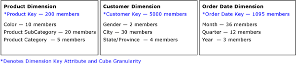
Figure 7   Product, Customer, and Order Date dimensions

Each dimension has four attributes. At the grain of the cube, there are 200 individual products, 5,000 individual customers, and 1,095 order dates. The maximum potential number of detailed values in this cube is the Cartesian product of these numbers: 200 * 5000 * 1095 or 109,500,000 theoretical combinations. This theoretical value is only possible if every customer buys every product on every day of every year, which is unlikely. In reality, the data distribution is likely a couple of orders of magnitude lower than the theoretical value. For this scenario, assume that the example cube has 1,095,000 combinations at the grain, a factor of 100 lower than the theoretical value.

Querying the cube at the grain is uncommon, given that such a large result set (1,095,000 cells) is probably not useful for end users. For any query that is not at the cube grain, the Storage Engine must perform an on-the-fly summarization of the detailed cells by the other dimension attributes, which can be costly to query performance. To optimize this summarization, Analysis Services uses aggregations to precalculate and store summaries of data during cube processing. With the aggregations readily available at query time, query performance can be improved greatly.

Continuing with the same cube example, if the cube contains an aggregation of sales by the month and product subcategory attributes, a query that requires sales by month by product subcategory can be directly satisfied by the aggregation without going to the fact data. The maximum number of cells in this aggregation is 720 (20 product subcategory members * 36 months, excluding the All attribute). While the actual number cells in the aggregation is again dependent on the data distribution, the maximum number of cells, 720, is considerably more efficient than summarizing values from 1,095,000 cells.

In addition, the benefit of the aggregation applies beyond those queries that directly match the aggregation. Whenever a query request is issued, the Storage Engine attempts to use any aggregation that can help satisfy the query request, including aggregations that are at a finer level of detail. For these queries, the Storage Engine simply summarizes the cells in the aggregation to produce the desired result set. For example, if you request sales data summarized by month and product category, the Storage Engine can quickly summarize the cells in the month and product subcategory aggregation to satisfy the query, rather than re-summarizing data from the lowest level of detail. To realize this benefit, however, requires that you have properly designed your dimensions with attribute relationships and natural hierarchies so that Analysis Services understands how attributes are related to each other. For more information on dimension design, see Optimizing the dimension design.

How the Storage Engine uses aggregations

To gain some insight into how the Storage Engine uses aggregations, you can use SQL Server Profiler to view how and when aggregations are used to satisfy queries. Within SQL Server Profiler, there are several events that describe how a query is fulfilled. The event that specifically pertains to aggregation hits is the Get Data From Aggregation event. Figure 8 displays a sample query and result set from an example cube.


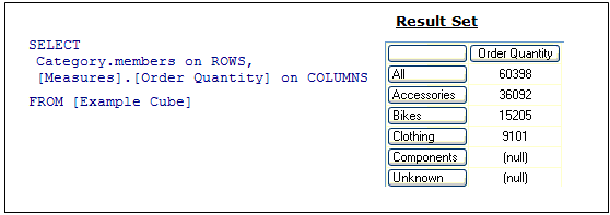
Figure 8   Sample query and result set

For the query displayed in Figure 8, you can use SQL Server Profiler to compare how the query is resolved in the following two scenarios:

  • Scenario 1—Querying against a cube where an aggregation satisfies the query request.
  • Scenario 2—Querying against a cube where no aggregation satisfies the query request.


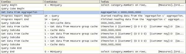
Figure 9   Scenario 1: SQL Server Profiler trace for cube with an aggregation hit

Figure 9 displays a SQL Server Profiler trace of the query’s resolution against a cube with aggregations. In the SQL Server Profiler trace, you can see the operations that the Storage Engine performs to produce the result set.

To satisfy the query, the following operations are performed:

  1. After the query is submitted, the Storage Engine gets data from Aggregation C 0000, 0001, 0000 as indicated by the Get Data From Aggregation event.

    Aggregation C is the name of the aggregation. Analysis Services assigns the aggregation with a unique name in hexadecimal format. Note that aggregations that have been migrated from earlier versions of Analysis Services use a different naming convention.

  2. In addition to the aggregation name, Aggregation C, Figure 9 displays a vector, 000, 0001, 0000 , that describes the content of the aggregation. More information on what this vector actually means is described in How to interpret aggregations.
  3. The aggregation data is loaded into the Storage Engine measure group cache.
  4. Once in the measure group cache, the Query Execution Engine retrieves the data from the cache and returns the result set to the client.


Figure 10   Scenario 2: SQL Server Profiler trace for cube with no aggregation hit

Figure 10 displays a SQL Server Profiler trace for the same query against the same cube but this time, the cube has no aggregations that can satisfy the query request.

To satisfy the query, the following operations are performed:

  1. After the query is submitted, rather than retrieving data from an aggregation, the Storage Engine goes to the detail data in the partition.
  2. From this point, the process is the same. The data is loaded into the Storage Engine measure group cache.
  3. Once in the measure group cache, the Query Execution Engine retrieves the data from the cache and returns the result set to the client.

To summarize these two scenarios, when SQL Server Profiler displays Get Data From Aggregation, this indicates an aggregation hit. With an aggregation hit, the Storage Engine can retrieve part or all of the data answer from the aggregation and does not need to go to the data detail. Other than fast response times, aggregation hits are a primary indication of a successful aggregation design.

To help you achieve an effective aggregation design, Analysis Services provides tools and techniques to help you create aggregations for your query workload. For more information on these tools and techniques, see Which aggregations are built in this white paper. Once you have created and deployed your aggregations, SQL Server Profiler provides excellent insight to help you monitor aggregation usage over the lifecycle of the application.

Why not create every possible aggregation?

Since aggregations can significantly improve query performance, you may wonder why not create every possible aggregation? Before answering this question, first consider what creating every possible aggregation actually means in theoretical terms.

Note that the goal of this theoretical discussion is to help you understand how aggregations work in an attribute-based architecture. It is not meant to be a discussion of how Analysis Services actually determines which aggregations are built. For more information on this topic, see Which aggregations are built in this white paper.

Generally speaking, an aggregation summarizes measures by a combination of attributes. From an aggregation perspective, for each attribute, there are two levels of detail: the attribute itself and the All attribute. Figure 11 displays the levels of detail for each attribute in the product dimension.


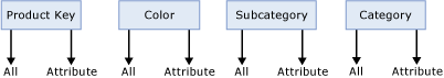
Figure 11   Attribute levels for the product dimension

With four attributes and two levels of detail (All and attribute), the total possible combination for the product dimension is 2*2*2*2 or 2^4 = 16 vectors or potential aggregations.


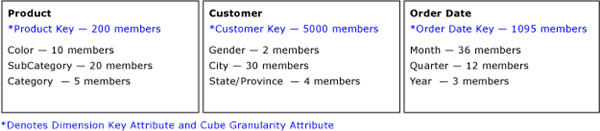
Figure 12   (3) dimensions with (4) attributes per dimension

If you apply this logic across all attributes displayed in Figure 12, the total number of possible aggregations can be represented as follows:

Total Number of Aggregations

2 (product key) *2 (color) *2 (product subcategory) * 2 (product category)*

2 (customer key) *2 (gender) *2 (city) *2 (state/province) *

2 (order date key) * 2 (month) * 2 (quarter)* 2 (year)

= 2^12

= 4096

Based on this example, the total potential aggregations of any cube can be expressed as 2^ (total number of attributes). While a cube with twelve attributes produces 4,096 theoretical aggregations, a large scale cube may have hundreds of attributes and consequently an exponential increase in the number of aggregations. A cube with 100 attributes, for example, would have 1.26765E+30 theoretical aggregations!

The good news is that this is just a theoretical discussion. Analysis Services only considers a small percentage of these theoretical aggregations, and eventually creates an even smaller subset of aggregations. As a general rule, an effective Analysis Services aggregation design typically contains tens or hundreds of aggregations, not thousands.

With that in mind, the theoretical discussion reminds us that as you add additional attributes to your cube, you are potentially increasing the number of aggregations that Analysis Services must consider. Furthermore, since aggregations are created at the time of cube processing, too many aggregations can negatively impact processing performance or require excessive disk space to store. As a result, ensure that your aggregation design supports the required data refresh timeline.

How to interpret aggregations

When Analysis Services creates an aggregation, each dimension is named by a vector, indicating whether the attribute points to the attribute or to the All level. The Attribute level is represented by 1 and the All level is represented by 0. For example, consider the following examples of aggregation vectors for the product dimension:

  • Aggregation By ProductKey Attribute
    = [Product Key]:1 [Color]:0 [Subcategory]:0 [Category]:0 or 1000

  • Aggregation By Category Attribute
    = [Product Key]:0 [Color]:0 [Subcategory]:0 [Category]:1 or 0001

  • Aggregation By ProductKey.All
    and Color.All and Subcategory.All and Category.All = [Product Key]:0 [Color]:0 [Subcategory]:0 [Category]:0 or 0000

To identify each aggregation, Analysis Services combines the dimension vectors into one long vector path, also called a subcube, with each dimension vector separated by commas.

The order of the dimensions in the vector is determined by the order of the dimensions in the cube. To find the order of dimensions in the cube, use one of the following two techniques. With the cube opened in SQL Server Business Intelligence Development Studio, you can review the order of dimensions in a cube on the Cube Structure tab. The order of dimensions in the cube is displayed in the Dimensions pane, on both the Hierarchies tab and the Attributes tab. As an alternative, you can review the order of dimensions listed in the cube XML file.

The order of attributes in the vector for each dimension is determined by the order of attributes in the dimension. You can identify the order of attributes in each dimension by reviewing the dimension XML file.

For example, the following subcube definition (0000, 0001, 0001) describes an aggregation for:

Product – All, All, All, All

Customer – All, All, All, State/Province

Order Date – All, All, All, Year

Understanding how to read these vectors is helpful when you review aggregation hits in SQL Server Profiler. In SQL Server Profiler, you can view how the vector maps to specific dimension attributes by enabling the Query Subcube Verbose event.

Which aggregations are built

To decide which aggregations are considered and created, Analysis Services provides an aggregation design algorithm that uses a cost/benefit analysis to assess the relative value of each aggregation candidate.

  • Aggregation Cost—The cost of an aggregation is primarily influenced by the aggregation size. To calculate the size, Analysis Services gathers statistics including source record counts and member counts, as well as design metadata including the number of dimensions, measures, and attributes. Once the aggregation cost is calculated, Analysis Services performs a series of tests to evaluate the cost against absolute cost thresholds and to evaluate the cost compared to other aggregations.
  • Aggregation Benefit—The benefit of the aggregation depends on how well it reduces the amount of data that must be scanned during querying. For example, if you have 1,000,000 data values that are summarized into an aggregation of fifty values, this aggregation greatly benefits query performance. Remember that Analysis Services can satisfy queries by using an aggregation that matches the query subcube exactly, or by summarizing data from an aggregation at a lower level (a more detailed level). As Analysis Services determines which aggregations should be built, the algorithm needs to understand how attributes are related to each other so it can detect which aggregations provide the greatest coverage and which aggregations are potentially redundant and unnecessary.

To help you build aggregations, Analysis Services exposes the algorithm using two tools: the Aggregation Design Wizard and the Usage-Based Optimization Wizard.

  • The Aggregation Design Wizard designs aggregations based on your cube design and data distribution. Behind the scenes, it selects aggregations using a cost/benefit algorithm that accepts inputs about the design and data distribution of the cube. The Aggregation Design Wizard can be accessed in either Business Intelligence Development Studio or SQL Server Management Studio.
  • The Usage-Based Optimization
    Wizard designs aggregations based on query usage patterns. The Usage-Based Optimization Wizard uses the same cost/benefit algorithm as the Aggregation Design Wizard except that it provides additional weighting to those aggregation candidates that are present in the Analysis Services query log. The Usage-Based Optimization Wizard can be accessed in either Business Intelligence Development Studio (BIDS) or SQL Server Management Studio. To use the Usage-Based Optimization Wizard, you must capture end-user queries and store the queries in a query log. To set up and configure the query log for an instance of Analysis Services, you can access a variety of configuration settings in SQL Server Management Studio to control the sampling frequency of queries and the location of the query log.

In those special scenarios when you require finer grained control over aggregation design, SQL Server Service Pack 2 samples includes an advanced Aggregation utility. Using this advanced tool, you can manually create aggregations without using the aggregation design algorithm. For more information on the Aggregation utility, see Appendix C.

How to impact aggregation design

To help Analysis Services successfully apply the aggregation design algorithm, you can perform the following optimization techniques to influence and enhance the aggregation design. (The sections that follow describe each of these techniques in more detail).

Suggesting aggregation candidates – When Analysis Services designs aggregations, the aggregation design algorithm does not automatically consider every attribute for aggregation. Consequently, in your cube design, verify the attributes that are considered for aggregation and determine whether you need to suggest additional aggregation candidates.     

Specifying statistics about cube data
To make intelligent assessments of aggregation costs, the design algorithm analyzes statistics about the cube for each aggregation candidate. Examples of this metadata include member counts and fact table counts. Ensuring that your metadata is up-to-date can improve the effectiveness of your aggregation design.

Adopting an aggregation design strategy – To help you design the most effective aggregations for your implementation, it is useful to adopt an aggregation design strategy that leverages the strengths of each of the aggregation design methods at various stages of your development lifecycle.

Suggesting aggregation candidates

When Analysis Services designs aggregations, the aggregation design algorithm does not automatically consider every attribute for aggregation. Remember the discussion of the potential number of aggregations in a cube? If Analysis Services were to consider every attribute for aggregation, it would take too long to design the aggregations, let alone populate them with data. To streamline this process, Analysis Services uses the Aggregation Usage property to determine which attributes it should automatically consider for aggregation. For every measure group, verify the attributes that are automatically considered for aggregation and then determine whether you need to suggest additional aggregation candidates.

The aggregation usage rules

An aggregation candidate is an attribute that Analysis Services considers for potential aggregation. To determine whether or not a specific attribute is an aggregation candidate, the Storage Engine relies on the value of the Aggregation Usage property. The Aggregation Usage property is assigned a per-cube attribute, so it globally applies across all measure groups and partitions in the cube. For each attribute in a cube, the Aggregation Usage property can have one of four potential values: Full, None, Unrestricted, and Default.

  • Full: Every aggregation for the cube must include this attribute or a related attribute that is lower in the attribute chain. For example, you have a product dimension with the following chain of related attributes: Product, Product Subcategory, and Product Category. If you specify the Aggregation Usage for Product Category to be Full, Analysis Services may create an aggregation that includes Product Subcategory as opposed to Product Category, given that Product Subcategory is related to Category and can be used to derive Category totals.
  • None—No aggregation for the cube may include this attribute.
  • Unrestricted—No restrictions are placed on the aggregation designer; however, the attribute must still be evaluated to determine whether it is a valuable aggregation candidate.
  • Default—The designer applies a default rule based on the type of attribute and dimension. As you may guess, this is the default value of the Aggregation Usage property.

The default rule is highly conservative about which attributes are considered for aggregation. Therefore, it is extremely important that you understand how the default rule works. The default rule is broken down into four constraints:

  1. Default Constraint 1Unrestricted for the Granularity and All Attributes – For the dimension attribute that is the measure group granularity attribute and the All attribute, apply Unrestricted. The granularity attribute is the same as the dimension’s key attribute as long as the measure group joins to a dimension using the primary key attribute.

    To help you visualize how Default Constraint 1 is applied, Figure 13 displays a product dimension with six attributes. Each attribute is displayed as an attribute hierarchy. In addition, three user hierarchies are included in the dimension. Within the user hierarchies, there are two natural hierarchies displayed in blue and one unnatural hierarchy displayed in grey. In addition to the All attribute (not pictured in the diagram), the attribute in yellow, Product Key, is the only aggregation candidate that is considered after the first constraint is applied. Product Key is the granularity attribute for the measure group.


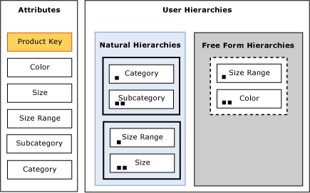
    Figure 13   Product dimension aggregation candidates after applying Default Constraint 1

  2. Default Constraint 2None for Special Dimension Types – For all attributes (except All) in many-to-many, nonmaterialized reference dimensions, and data mining dimensions, use None. The product dimension in Figure 13 is a standard dimension. Therefore it is not affected by constraint 2. For more information on many-to-many and reference dimensions, see Complex dimension relationships.
  3. To identify the natural hierarchies, Analysis Services scans each user hierarchy starting at the top level and then moves down through the hierarchy to the bottom level. For each level, it checks whether the attribute of the current level is linked to the attribute of the next level via a direct or indirect attribute relationship, for every attribute that pass the natural hierarchy test, apply Unrestricted, except for nonaggregatable attributes, which are set to Full.

  4. Default Constraint 4None For Everything Else. For all other dimension attributes, apply None. In this example, the color attribute falls into this bucket since it is only exposed as an attribute hierarchy.

Figure 14 displays what the Product dimension looks like after all constraints in the default rule have been applied. The attributes in yellow highlight the aggregation candidates.

  • As a result of Default Constraint 1, the Product Key and All attributes have been identified as candidates.
  • As a result of Default Constraint 3, the Size, Size Range, Subcategory, and Category attributes have also been identified as candidates.
  • After Default Constraint 4 is applied, Color is still not considered for any aggregation.


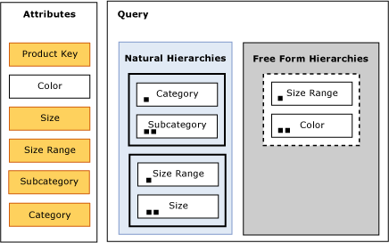
Figure 14   Product dimension aggregation candidates after all application of all default constraints

While the diagrams are helpful to visualize what happens after the each constraint is applied, you can view the specific aggregation candidates for your own implementation when you use the Aggregation Design Wizard to design aggregations.

Figure 15 displays the Specify Object Counts page of the Aggregation Design Wizard. On this Wizard page, you can view the aggregation candidates for the Product dimension displayed in Figure 14. The bold attributes in the Product Dimension are the aggregation candidates for this dimension. The Color attribute is not bold because it is not an aggregation candidate. This Specify Object Counts page is discussed again in Specifying statistics about cube metadata, which describes how you can update statistics to improve aggregation design.


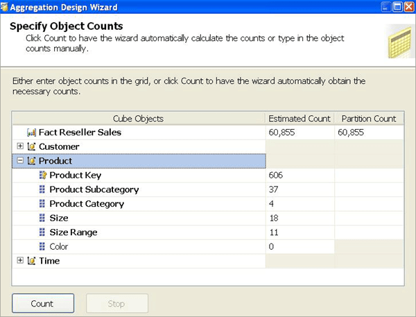
Figure 15   Aggregation candidates in the Aggregation Design Wizard

Influencing aggregation candidates

In light of the behavior of the Aggregation Usage property, following are some guidelines that you can adopt to influence the aggregation candidates for your implementation. Note that by making these modifications, you are influencing the aggregation candidates, not guaranteeing that a specific aggregation is going to be created. The aggregation must still be evaluated for its relative cost and benefit before it is created. The guidelines have been organized into three design scenarios:

  • Dimensions with no user hierarchies—If your dimension ONLY has attribute hierarchies with no user-defined hierarchies, by default the only attribute that is considered for aggregation is the cube granularity attribute plus the All attribute. As such, you may want to consider adding some natural hierarchies to your design. In addition to the Aggregation Usage benefits, your users may enjoy the analysis experience of using predefined navigation paths.
  • Attribute only exposed in an attribute hierarchy—If a given attribute is only exposed as an attribute hierarchy such as Color in Figure 14, you may want to change its Aggregation Usage property as follows:
    • Change the value of the Aggregation Usage property from Default to Unrestricted if the attribute is a commonly used attribute or if there are special considerations for improving the performance in a particular pivot or drilldown. For example, if you have highly summarized scorecard style reports, you want to ensure that the users experience good initial query response time before drilling around into more detail.
    • While setting the Aggregation Usage property of a particular attribute hierarchy to Unrestricted is appropriate is some scenarios, do not be tempted to set all of your attribute hierarchies to Unrestricted. While this scenario seems reasonable, you may quickly find yourself in a position where the Wizard takes a very long time to consider all of the possible candidates and create an aggregation design. In large cubes, the Wizard can take at least an hour to complete the design and considerably much more time to process. As such, you should set the property to Unrestricted only for the commonly queried attribute hierarchies. The general rule is five to ten Unrestricted attributes per dimension.
    • Change the value of the Aggregation Usage property from Default to Full in the unusual case that it is used in virtually every query you want to optimize. This is a very rare case and should only be used for attributes that have a relatively small number of members.
  • Infrequently used attributes—For attributes participating in natural hierarchies, you may want to change the Aggregation Usage property from Default to None if users would only infrequently use it. Using this approach can help you reduce the aggregation space and get to the five to ten Unrestricted attributes per dimension. For example, you may have certain attributes that are only used by a few advanced users who are willing to accept slightly slower performance. In this scenario, you are essentially forcing the aggregation design algorithm to spend time building only the aggregations that provide the most benefit to the majority of users. Another example where you may want to consider setting the Aggregation Usage property to None is when you have a natural hierarchy where the number of members from one level to the next level is almost identical. For example, if you have 20 product subcategories and 18 product categories, it may make sense to set the product category attribute to None since the I/O penalty of aggregating 20 members up to 18 members is negligible. Generally speaking, if the data does not support at least a 2:1 ratio, you should consider setting the Aggregation Usage to None.
Specifying statistics about cube data

Once the aggregation design algorithm has identified the aggregation candidates, it performs a cost/benefit analysis of each aggregation. In order to make intelligent assessments of aggregation costs, the design algorithm analyzes statistics about the cube for each aggregation candidate. Examples of this metadata include member counts and fact table record counts. Ensuring that your metadata is up-to-date can improve the effectiveness of your aggregation design.

You can define the fact table source record count in the EstimatedRows property of each measure group, and you can define attribute member count in the EstimatedCount property of each attribute.

You can modify these counts in the Specify Counts page of the Aggregation Design Wizard as displayed in Figure 16.


Figure 16   Specify object counts in the Aggregation Design Wizard

If the count is NULL (i.e., you did not define it during design), clicking the Count button populates the counts for each aggregation candidate as well as the fact table size. If the count is already populated, clicking the Count button does not update the counts. Rather you must manually change the counts either in the dialog box or programmatically. This is significant when you design aggregations on a small data set and then move the cube to a production database. Unless you update the counts, any aggregation design is built by using the statistics from the development data set.

In addition, when you use multiple partitions to physically divide your data, it is important that the partition counts accurately reflect the data in the partition and not the data across the measure group. So if you create one partition per year, the partition count for the year attribute should be 1. Any blank counts in the Partition Count column use the Estimated Count values, which apply to the entire fact table.

Using these statistics, Analysis Services compares the cost of each aggregation to predefined cost thresholds to determine whether or not an aggregation is too expensive to build. If the cost is too high, it is immediately discarded. One of the most important cost thresholds is known as the one-third rule. Analysis Services never builds an aggregation that is greater than one third of the size of the fact table. In practical terms, the one-third rule typically prevents the building of aggregations that include one or more large attributes.

As the number of dimension members increases at deeper levels in a cube, it becomes less likely that an aggregation will contain these lower levels because of the one-third rule. The aggregations excluded by the one-third rule are those that would be almost as large as the fact level itself and almost as expensive for Analysis Services to use for query resolution as the fact level. As a result, they add little or no value.

When you have dimensions with a large number of members, this threshold can easily be exceeded at or near the leaf level. For example, you have a measure group with the following design:

  • Customer dimension with 5,000,000 individual customers organized into 50,000 sales districts and 5,000 sales territories
  • Product dimension with 10,000 products organized into 1,000 subcategories and 30 categories
  • Time dimension with 1,095 days organized into 36 months and 3 years
  • Sales fact table with 12,000,000 sales records

If you model this measure group using a single partition, Analysis Services does not consider any aggregation that exceeds 4,000,000 records (one third of the size of the partition). For example, it does not consider any aggregation that includes the individual customer, given that the customer attribute itself exceeds the one-third rule. In addition, it does not consider an aggregation of sales territory, category, and month since the total number of records of that aggregation could potentially be 5.4 million records consisting of 5,000 sales territories, 30 categories, and 36 months.

If you model this measure group using multiple partitions, you can impact the aggregation design by breaking down the measure group into smaller physical components and adjusting the statistics for each partition.

For example, if you break down the measure group into 36 monthly partitions, you may have the following data statistics per partition:

  • Customer dimension has 600,000 individual customers organized into 10,000 sales districts and 3,000 sales territories
  • Product dimension with 7,500 products organized into 700 subcategories and 25 categories
  • Time dimension with 1 month and 1 year
  • Sales fact table with 1,000,000 sales records

With the data broken down into smaller components, Analysis Services can now identify additional useful aggregations. For example, the aggregation for sales territory, category, and month is now a good candidate with (3000 sales territories *25 categories *1 month) or 75,000 records which is less than one third of the partition size of 1,000,000 records. While creating multiple partitions is helpful, it is also critical that you update the member count and partition count for the partition as displayed in Figure 16. If you do not update the statistics, Analysis Services will not know that the partition contains a reduced data set. Note that this example has been provided to illustrate how you can use multiple partitions to impact aggregation design. For practical partition sizing guidelines, including the recommended number of records per partition, see Designing partitions in this white paper.

Note that you can examine metadata stored on, and retrieve support and monitoring information from, an Analysis Services instance by using XML for Analysis (XMLA) schema rowsets. Using this technique, you can access information regarding partition record counts and aggregation size on disk to help you get a better sense of the footprint of Analysis Services cubes.

Adopting an aggregation design strategy

The goal of an aggregation design strategy is to help you design and maintain aggregations throughout your implementation lifecycle. From an aggregation perspective, the cube lifecycle can be broken down into two general stages: initial aggregation design and ongoing tuning based on query patterns.

Initial Aggregation Design

The most effective aggregation designs are those that are customized for the querying patterns of your user base. Unfortunately, when you initially deploy a cube, you probably will not have query usage data available. As such, it is not possible to use the Usage-Based Optimization Wizard. However, because Analysis Services generally resolves user queries faster with some aggregations than with none, you should initially design a limited number of aggregations by using the Aggregation Design Wizard. The number of initial aggregations that you should design depends on the complexity and size of the cube (the fact size).

  • Small cubes—With a small cube, an effective aggregation strategy is to initially design aggregations using the Aggregation Design Wizard to achieve a 20 to 30 percent increase in performance. Note that if the design has too many attributes to consider for aggregation, there is a chance that the Aggregation Design Wizard will stop before reaching the designed percent performance improvement and the user interface may not visibly show any percent performance increase. In this scenario, the large number of attributes has resulted in many possible aggregations, and the number of aggregations that have actually been created are a very small percentage of the total possible aggregations.
  • Large and complex cubes—With a large and complex cube, it takes Analysis Services a long time just to design a small percentage of the possible aggregations. Recall that the number of theoretical aggregations in a cube can be expressed as 2^ (total number of Unrestricted attributes). A complex cube with five dimensions that each contain eight attributes has 2^40 or 1.1 trillion aggregation candidates (given that every attribute is an aggregation candidate). With this number, if you assume that the Aggregation Design Wizard can examine 1000 aggregations per second (which is a very generous estimate), it will take the Aggregation Design Wizard approximately 35 years to consider a trillion possible aggregations. Furthermore, a large number of aggregations takes a long time to calculate and consumes a large amount of disk space. While this is a theoretical example, an effective approach with real world cubes that are large and complex is to initially design aggregations to achieve a small performance increase (less than 10 percent and possibly even 1 or 2 percent with very complex cubes) and then allow the Aggregation Design Wizard to run for no more than 15 minutes.
  • Medium complexity cubes—With a medium-complexity cube, design aggregations to achieve a 10 to 20 percent increase in performance. Then, allow the wizard to run for no more than 15 minutes. While it is difficult to define what constitutes a high-complexity cube versus a medium-complexity cube, consider this general guideline: a high-complexity cube is a cube contains more than ten Unrestricted attributes in any given dimension.

Before you create initial aggregations with the Aggregation Design Wizard, you should evaluate the application Aggregation Usage property and modify its value as necessary to minimize aggregations that are rarely used and to maximize the probability of useful aggregations. Using Aggregation Usage is equivalent to providing the aggregation algorithm with “hints” about which attributes are frequently and infrequently queried. For specific guidelines on modifying the Aggregation Usage property, see Influencing aggregation candidates.

After you design aggregations for a given partition, it is a good practice to evaluate the size of the aggregation files. The total size of all aggregation files for a given partition should be approximately one to two times the size of the source fact table. If the aggregations are greater than two times the size of the fact table, you are likely spending a long time processing your cube to build relatively large aggregation files. During querying, you can potentially experience performance issues when large aggregation files cannot be effectively loaded into memory due to lack of system resources. If you experience these issues, it is good practice to consider reducing the number of aggregation candidates.

Ongoing tuning based on query patterns

After users have queried the cube for a sufficient period of time to gather useful query pattern data in the query log (perhaps a week or two), use the Usage-Based Optimization Wizard to perform a usage-based analysis for designing additional aggregations that would be useful based on actual user query patterns. You can then process the partition to create the new set of aggregations. As usage patterns change, use the Usage-Based Optimization Wizard to update additional aggregations.

Remember that to use the Usage-Based Optimization Wizard, you must capture end-user queries and store the queries in a query log. Logging queries requires a certain amount of overhead so it is generally recommended that you turn off logging and then turn it back on periodically when you need to tune aggregations based on query patterns.

As an alternative to using the Usage-Based Optimization Wizard, if you require finer grained control over aggregation design, SQL Server Service Pack 2 samples includes an advanced Aggregation Utility that allows you to create specific aggregations from the query log without using the aggregation design algorithm. For more information on the Aggregation Utility, see Appendix C.

Using partitions to enhance query performance

Partitions separate measure group data into physical units. Effective use of partitions can enhance query performance, improve processing performance, and facilitate data management. This section specifically addresses how you can use partitions to improve query performance. The Using partitions to enhance processing performance section discusses the processing and data management benefits of partitions.

How partitions are used in querying

When you query a cube, the Storage Engine attempts to retrieve data from the Storage Engine cache. If no data is available in the cache, it attempts to retrieve data from an aggregation. If no aggregation is present, it must go to the fact data. If you have one partition, Analysis Services must scan though all of the fact data in the partition to find the data that you are interested in. While the Storage Engine can query the partition in parallel and use bitmap indexes to speed up data retrieval, with just one partition, performance is not going to be optimal.

As an alternative, you can use multiple partitions to break up your measure group into separate physical components. Each partition can be queried separately and the Storage Engine can query only the partition(s) that contain the relevant data.


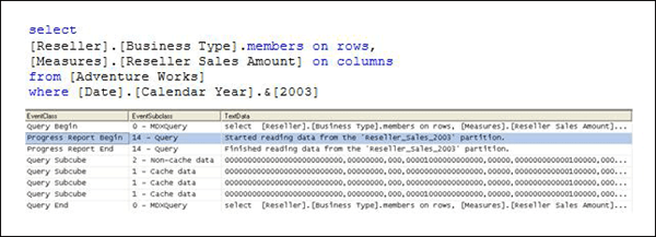
Figure 17   Intelligent querying by partitions

Figure 17 displays a query requesting Reseller Sales Amount by Business Type from a cube called Adventure Works as well as the SQL Server Profiler trace that describes how the query was satisfied. The Reseller Sales measure group of the Adventure Works cube contains four partitions: one for each year. Because the query slices on 2003, the Storage Engine can go directly to the 2003 Reseller Sales partition and does not have to scan data from other partitions. The SQL Server Profiler trace for this query demonstrates how the query needs to read data only from the 2003 Reseller Sales partition.

Designing partitions

If you have some idea how users query the data, you can partition data in a manner that matches common queries. This may be somewhat difficult if user queries do not follow common patterns. A very common choice for partitions is to select an element of time such as day, month, quarter, year or some combination of time elements. Many queries contain a time element, so partitioning by time often benefits query performance.

When you set up your partitions, you must bind each partition to a source table, view, or source query that contains the subset of data for that partition. For MOLAP partitions, during processing Analysis Services internally identifies the slice of data that is contained in each partition by using the Min and Max DataIDs of each attribute to calculate the range of data that is contained in the partition. The data range for each attribute is then combined to create the slice definition for the partition. The slice definition is persisted as a subcube. Knowing this information, the Storage Engine can optimize which partitions it scans during querying by only choosing those partitions that are relevant to the query. For ROLAP and proactive caching partitions, you must manually identify the slice in the properties of the partition.

As you design partitions, use the following guidelines for creating and managing partitions:

  • When you decide how to break down your data into partitions, you are generally weighing out partition size vs. number of partitions. Partition size is a function of the number of records in the partition as well as the size of the aggregation files for that partition. Even though the segments in a partition are queried in parallel, if the aggregation files for a partition cannot be effectively managed in memory, you can see significant performance issues during querying.
  • In general. the number of records per partition should not exceed 20 million. In addition, the size of a partition should not exceed 250 MB. If the partition exceeds either one of these thresholds, consider breaking the partition into smaller components to reduce the amount of time spent scanning the partition. While having multiple partitions is generally beneficial, having too many partitions, e.g., greater than a few hundred, can also affect performance negatively.
  • If you have several partitions that are less than 50 MB or 2 million records per partition, consider consolidating them into one partition. In addition, it is generally not a good practice to create a partition that has less than 4,096 records. In this scenario, given that the record count is so small, the Storage Engine does not create aggregations or indexes for the partition and therefore does not set the auto-slice. Note that this record count threshold is controlled by the IndexBuildThreshold property in the msmdsrv.ini file. Falling below this threshold is generally not an issue in production environments since partition data sets are typically much larger than 4,096 records.
  • When you define your partitions, remember that they do not have to contain uniform datasets. For example, for a given measure group, you may have three yearly partitions, 11 monthly partitions, three weekly partitions, and 1–7 daily partitions. The value of using heterogeneous partitions with different levels of detail is that you can more easily manage the loading of new data without disturbing existing partitions. In addition, you can design aggregations for groups of partitions that share the same level of detail (more information on this in the next section).
  • Whenever you use multiple partitions for a given measure group, you must ensure that you update the data statistics for each partition. More specifically, it is important to ensure that the partition data and member counts accurately reflect the specific data in the partition and not the data across the entire measure group. For more information on how to update partition counts, see Specifying statistics about cube data.
  • For distinct count measure groups, consider specifically defining your partitions to optimize the processing and query performance of distinct counts. For more information on this topic, see Optimizing distinct count.
Aggregation considerations for multiple partitions

For each partition, you can use a different aggregation design. By taking advantage of this flexibility, you can identify those data sets that require higher aggregation design. While the flexibility can definitely help you enhance performance, too many aggregation designs across your partitions can introduce overhead.

To help guide your aggregation design, the following are general guidelines for you to consider. When you have less than ten partitions, you should typically have no more than two aggregation designs per measure group. With less than 50 partitions, you typically want no more than three aggregation designs per measure group. For greater than 50 partitions, you want no more than four aggregation designs.

While each partition can have a different aggregation design, it is a good practice to group your partitions based on the data statistics of the partition so that you can apply a single aggregation design to a group of similar partitions.

Consider the following example. In a cube with multiple monthly partitions, new data may flow into the single partition corresponding to the latest month. Generally that is also the partition most frequently queried. A common aggregation strategy in this case is to perform Usage-Based Optimization to the most recent partition, leaving older, less frequently queried partitions as they are.

The newest aggregation design can also be copied to a base partition. This base partition holds no data—it serves only to hold the current aggregation design. When it is time to add a new partition (for example, at the start of a new month), the base partition can be cloned to a new partition. When the slice is set on the new partition, it is ready to take data as the current partition. Following an initial full process, the current partition can be incrementally updated for the remainder of the period. For more information on processing techniques, see Refreshing partitions efficiently.


Writing efficient MDX

When the Query Execution Engine executes an MDX query, it translates the query into Storage Engine data requests and then compiles the data to produce a query result set.

During query execution, the Query Execution Engine also executes any calculations that are directly or indirectly referenced, such as calculated members, semi-additive measures, and MDX Script scope assignments. Whenever you directly or indirectly reference calculations in your query, you must consider the impact of the calculations on query performance.

This section presents techniques for writing efficient MDX statements in common design scenarios. The section assumes that the reader has some knowledge of MDX.

Specifying the calculation space

When you need to create MDX calculations that apply business rules to certain cells in a cube, it is critical to write efficient MDX code that effectively specifies the calculation space for each rule.

Before you learn about these MDX coding techniques, it is important to be familiar with some common scenarios where conditional business rules are relevant. Following is a description of a growth calculation where you want to apply unique rules to different time periods. To calculate growth from a prior period, you may think that the logical expression for this calculation is current period minus prior period. In general, this expression is valid; however, it is not exactly correct in the following three situations.

  • The First Period—In the first time period of a cube, there is no prior period. Since the prior period does not exist for the first period, the expression of current period minus prior period evaluates to current period, which can be somewhat misleading. To avoid end-user confusion, for the prior period, you may decide to apply a business rule that replaces the calculation with NULL.
  • The All Attribute—You need to consider how the calculation interacts with the All. In this scenario, the calculation simply does not apply to the All, so you decide to apply a rule that sets the value for All to NA.
  • Future Periods—For time periods that extend past the end of the data range, you must consider where you want the calculation to stop. For example, if your last period of data is December of 2006, you want to use a business rule to only apply the calculation to time periods before and including December of 2006.

Based on this analysis, you need to apply four business rules for the growth from prior period calculation. Rule 1 is for the first period, rule 2 is for the All, rule 3 is for the future time periods and rule 4 is for the remaining time periods. The key to effectively applying these business rules is to efficiently identify the calculation space for each rule. To accomplish this, you have two general design choices:

  • You can create a calculated member with an IIF statement that uses conditional logic to specify the calculation space for a given period.
  • Alternatively you can create a calculated member and use an MDX Script scope assignment to specify the calculation space for a given period.

In a simple cube with no other calculations, the performance of these two approaches is approximately equal. However, if the calculated member directly or indirectly references any other MDX calculations such as semi-additive measures, calculated members, or MDX Script scope assignments, you can definitely see a performance difference between the two approaches. To see how MDX Script scope assignments can be used to perform the growth calculation, you can use the Business Intelligence Wizard to generate time intelligence calculations in your cube.

To better understand the performance benefit of the scope assignment technique used by the Business Intelligence Wizard, consider the following illustrative example of an effective scope assignment. You require a new calculated member called Weekend Gross Profit. The Weekend Gross Profit is derived from the Gross Profit calculated member. To calculate the Weekend Gross Profit, you must sum the Gross Profit calculated member for the days in a sales weekend. This seems easy enough but there are different business rules that apply to each sales territory to as follows:

  • For all of the stores in the North America sales territory, the Weekend Gross Profit should sum the Gross Profit for days 5, 6, and 7, i.e., Friday, Saturday, and Sunday.
  • For all of the stores in the Pacific sales territory, the Weekend Gross Profit should be NULL. You want to set it to NULL because the Pacific territory is in the process of closing of all of its stores and the Gross Profit numbers are significantly skewed due to their weekend clearance sales.
  • For all other territories, the Weekend Gross Profit should sum the Gross Profit for days 6 and 7, i.e., Saturday and Sunday.

To satisfy the conditions of this scenario, following are two design options that you can choose.

Option 1Calculated Member

You can use a calculated member with an IIF statement to apply the conditional summing of Gross Profit. In this scenario, the Query Execution Engine must evaluate the calculation space at runtime on a cell-by-cell basis based on the IIF specification. As a result, the Query Execution Engine uses a less optimized code path to execute the calculation that increases query response time.


with member [Option 1 Weekend Gross Profit] as

iif (ancestor([Sales Territory].[Sales Territory].CurrentMember,

[Sales Territory].[Sales Territory].[Group])

IS [Sales Territory].[Sales Territory].[Group].&[North America],

Sum({[Date].[Day of Week].&[5],

[Date].[Day of Week].&[6],

[Date].[Day of Week].&[7]},

[Measures].[Reseller Gross Profit]),

iif (ancestor([Sales Territory].[Sales Territory].CurrentMember,

[Sales Territory].[Sales Territory].[Group])

IS [Sales Territory].[Sales Territory].[Group].&[Pacific],

NULL,

Sum({[Date].[Day of Week].&[6],

[Date].[Day of Week].&[7]},

[Measures].[Reseller Gross Profit])))


Option 2—Scope assignment with a Calculated Member

In Option 2, you use a calculated member with a scope assignment to apply the conditional summing of Gross Profit.


CREATE MEMBER CURRENTCUBE.[MEASURES].[Option 2 Weekend Gross Profit] AS

Sum({[Date].[Day of Week].&[7],

[Date].[Day of Week].&[6] },

[Measures].[Reseller Gross Profit]);


Scope ([Option 2 Weekend Gross Profit],

Descendants([Sales Territory].[Sales Territory Group].&[North

America]));

This = Sum({[Date].[Day of Week].&[7],

[Date].[Day of Week].&[6],

[Date].[Day of Week].&[5] },

[Measures].[Reseller Gross Profit]);

End Scope;


Scope ([Option 2 Weekend Gross Profit],

Descendants([Sales Territory].[Sales Territory Group].&[Pacific]));

This = NULL;

End Scope;

In this example, this option is significantly faster than the first option. The reason this option is faster is because the two scope subcube definitions (the left hand side of each scope assignment) enable the Query Execution Engine to know ahead of time the calculation space for each business rule. Using this information, the Query Execution Engine can select an optimized execution path to execute the calculation on the specified range of cells. As a general rule, it is a best practice to always try to simplify calculation expressions by moving the complex parts into multiple Scope definitions whenever possible.

Note that in this Scope assignment, the Descendants function represents the Analysis Services 2000 approach to using MDX functions to navigate a dimension hierarchy. An alternative approach in Analysis Services 2005 is to simply use Scope with the attribute hierarchies. So instead of using Scope (Descendants([Sales Territory].[Pacific])), you can use Scope ([Sales Territory].[Pacific]).

To enhance performance, wherever possible, use the scope subcube definition to narrowly define the calculation space. While this is the ideal scenario, there are situations where it is not possible. The most common scenario is when you need to define a calculation on an arbitrary collection of cells ([Measures].[Reseller Sales Amount] >500). This type of expression is not allowed in the scope subcube definition since the definition must be static. In this scenario, the solution is to define a broader calculation space in the scope definition, and then use the scope MDX expression (the right hand side of the scope assignment) to narrow down the cube space using the IIF statement. The following is an example of how this statement can be structured to apply a weighting factor to the North American sales:


SCOPE ([Measures].[Sales Amount],

[Sales Territory].[Sales Territory].[Group].&[North America])

THIS =

IIF ([Measures].[Sales Amount] > 1000, [Measures].[Sales Amount],

[Measures].[Sales Amount]*1.2);

END SCOPE


From a performance perspective, MDX scope assignments provide an efficient alternative to using IIF to apply unique business rules to certain cells in a cube. Whenever you need to conditionally apply calculations, you should consider this approach.

Removing empty tuples

When you write MDX statements that use a set function such as Crossjoin, Descendants, or Members, the default behavior of the function is to return both empty and nonempty tuples. From a performance perspective, empty tuples can not only increase the number of rows and/or columns in your result set, but they can also increase query response time.

In many business scenarios, empty tuples can be removed from a set without sacrificing analysis capabilities. Analysis Services provides a variety of techniques to remove empty tuples depending on your design scenario.

Analysis Services ground rules for interpreting null values

Before describing these techniques, it is important to establish some ground rules about how empty values are interpreted in various design scenarios.

  • Missing fact table records—Earlier in the white paper, it was stated that only records that are present in the relational fact table are stored in the partition. For example, a sales fact table only stores records for those customers with sales for a particular product. If a customer never purchased a product, a fact table record will not exist for that customer and product combination. The same holds true for the Analysis Services partition. If a fact table record does not exist for a particular combination of dimension members, the cube cells for these dimension members are considered empty.
  • Null values in measures—For each fact table measure that is loaded into the partition, you can decide how Analysis Services interprets null values. Consider the following example. Your sales fact table contains a record that has a sales amount of 1000 and a discount amount of null. When discount is loaded into the cube, by default it is interpreted as a zero, which means that it is not considered empty. How Analysis Services interprets null values is controlled by a property called NullProcessing. The NullProcessing property is set on a measure-by-measure basis. By default, it is set to Automatic which means that Analysis Services converts the null values to zero. If you want to preserve the null value from the source system, such as in the example of the discount measure, configure the NullProcessingProperty of that measure to Preserve instead of Automatic.
  • Null values in calculations—In calculations, it is important to understand how Nulls are evaluated. For example, 1 minus Null equals 1, not Null. In this example, the Null is treated like a zero for calculation purposes. which may or may not be what you want to use. To explicitly test whether a tuple is null, use the ISEmpty function within an IIF statement to conditionally handle empty tuples.
  • Empty members—When writing calculations that reference dimension members, you may need to handle scenarios where specific members do not exist, such as the parent of the All. In this scenario, the ISEmpty function is not appropriate as it tests for empty cells. Rather in this scenario you want to use the IS operator to test whether the member IS NULL.


General techniques for removing empty tuples

The following describes the most general techniques for removing empty tuples:

  • Non Empty Keyword—When you want to remove empty rows or columns from the axes of an MDX query, you can use the NON EMPTY keyword. Most client applications use the NON EMPTY keyword to remove empty cells in query result sets. The NON EMPTY keyword is applied to an axis and takes effect after the query result set is determined, i.e., after the Query Execution Engine completes the axis tuples with the current members taken from the rows axis, columns axis, and WHERE clause (as well as the default members of the attribute hierarchies not referenced in the query).

    Consider the following example displayed in Figure 18. Note that only a subset of the query results is shown.


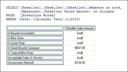
    Figure 18 – Query without Non Empty Keyword


In Figure 18, the rows axis returns a complete list of resellers, regardless of whether or not they have sales in 2003. For each reseller, the columns axis displays the reseller’s 2003 sales. If the reseller had no sales in 2003, the reseller is still returned in the list, it is just returned with a (null) value.

To remove resellers who do not have sales in 2003, you can use the NON EMPTY keyword as displayed in Figure 19. Note that only a subset of the query results is shown.


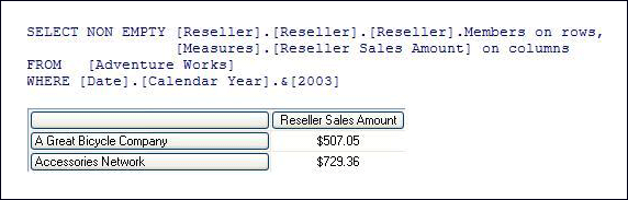
Figure 19 – Query with Non Empty Keyword


In Figure 19, the NON EMPTY keyword removes the resellers that do not have sales, i.e., null sales for 2003. To apply the NON EMPTY keyword, the Query Execution Engine must completely evaluate all cells in the query before it can remove the empty tuples.

If the query references a calculated member, the Query Execution Engine must evaluate the calculated member for all cells in the query and then remove the empty cells. Consider the example displayed in Figure 20. Note that only a subset of the query results is shown. In this example, you have modified the reseller query, replacing Reseller Sales Amount with the calculated measure Prior Year Variance. To produce the query result set, Analysis Services first obtains a complete set of resellers and then removes those resellers that have an empty prior year variance.


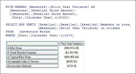
Figure 20 – Query with Non Empty Keyword and Calculated Measure


Given the ground rules about null interpretation, it is necessary to point out when the prior year variance is going to be null.

  • Acceptable Sales & Service has no sales in 2003 but has sales of $838.92 in 2002. The Prior Year Variance calculation is null minus $838.92 which evaluates to -$838.92. Since the value is not null, that reseller is returned in the result set.
  • Accessories Network has $729.36 sales in 2003 but no sales in 2002. The Prior Year Variance calculation is $729.36 minus null which evaluates to $729.36. Since the value is not null, the reseller is returned in the result set.
  • If a reseller has no sales in either 2003 or 2002, the calculation is null minus null, which evaluates to null. The reseller is removed from the result set.
  • NonEmpty Function—The NonEmpty function, NonEmpty(), is similar to the NON EMPTY keyword but it provides additional flexibility and more granular control. While the NON EMPTY keyword can only be applied to an axis, the NonEmpty function can be applied to a set. This is especially useful when you are writing MDX calculations.

    As an additional benefit, the NonEmpty function allows you use an MDX expression to evaluate the empty condition against a business rule. The business rule can reference any tuple, including calculated members. Note that if you do not specify the MDX expression in the NonEmpty function, the NonEmpty function behaves just like the NON EMPTY keyword, and the empty condition is evaluated according to the context of the query.

    Continuing with the previous examples regarding resellers, you want to change the previous queries to apply your own business rule that decides whether or not a reseller is returned in the query. The business rule is as follows. You want a list of all resellers that had a sale in 2002. For each of these resellers, you only want to display their sales for 2003. To satisfy this requirement, you use the query displayed in Figure 21. Note that only a subset of the query results is shown.


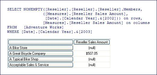
Figure 21 Query with NonEmpty Function


In this query, the NonEmpty function returns those resellers that had a sale in 2002. For each of these resellers, their 2003 sales are displayed. Note that query produces a different list of resellers than the resellers returned in the NON EMPTY keyword example. The Accessories Network reseller has been removed because it only has sales in 2003 with no sales in 2002.

Note that an alternative way to write this query is to use the FILTER expression, such as the following:


SELECT FILTER ([Reseller].[Reseller].[Reseller].Members,

NOT ISEmpty(([Measures].[Reseller Sales Amount],

[Date].[Calendar Year].&[2002]))) on rows,

[Measures].[Reseller Sales Amount] on columns

FROM [Adventure Works]    

WHERE [Date].[Calendar Year].&[2003]


In this query, FILTER is used to return only those resellers who had a sale in 2002. FILTER was commonly used in prior versions of Analysis Services. For simple expressions like the one depicted in the above example, Analysis Services actually re-writes the query behind-the-scenes using the NonEmpty function. For other more complicated expressions, it is advisable to use the NonEmpty function in place of the FILTER expression. In Analysis Services 2005, the NonEmpty function provides a more optimized alternative to using the FILTER expression to check for empty cells.

As you use NON EMPTY keyword and NonEmpty function to remove empty tuples, consider the following guidelines:

  • The NonEmpty function and NON EMPTY keyword will have approximately the same performance when the parameters passed to NonEmpty function coincide with the query axes of a NON EMPTY keyword query.
  • In common scenarios, Non Empty is normally used instead of NonEmpty() at the top level of SELECT query axes.
  • In calculations or query sub expressions, NonEmpty() is the recommended approach to achieve similar semantics. When using NonEmpty(), pay extra attention to making sure that the current cell context used by NonEmpty() is the intended one, possibly by specifying additional sets and members as the second parameter of the function.
  • Non_Empty_Behavior (NEB)—Whether or not an expression resolves to null is important for two major reasons. First, most client applications use the NON EMPTY key word in a query. If you can tell the Query Execution Engine that you know an expression will evaluate to null, it does not need to be computed and can be eliminated from the query results before the expression is evaluated. Second, the Query Execution Engine can use the knowledge of a calculation’s Non_Empty_Behavior (NEB) even when the NON EMPTY keyword is not used. If a cell’s expression evaluates to null, it does not have to be computed during query evaluation.

    Note that the current distinction between how the Query Execution Engine uses an expression’s NEB is really an artifact of the Query Execution Engine design. This distinction indicates whether one or both optimizations are used, depending how the NEB calculation property is defined. The first optimization is called NonEmpty Optimization and the second optimization is called Query Execution Engine Optimization.

    When an expression’s NEB is defined, the author is guaranteeing that the result is null when the NEB is null and consequently the result set is not null when NEB is not null. This information is used internally by the Query Execution Engine to build the query plan.

    To use NEB for a given calculation, you provide an expression that defines the conditions under which the calculation is guaranteed to be empty. The reason why NEB is an advanced setting is because it is often difficult to correctly identify the conditions under which the calculation is guaranteed to be empty. If you incorrectly set NEB, you will receive incorrect calculation results. As such, the primary consideration of using NEB is to ensure first and foremost that you have defined the correct expression, before taking into account any performance goals.

    The NEB expression can be a fact table measure, a list of two or more fact table measures, a tuple, or a single measure set. To help you better understand which optimizations are used for each expression; consider the guidelines in Table 2.

    Table 2   NEB guidelines


Calculation Type 

NEB
Expressions

Query Execution Engine Optimization Support 

NonEmpty Optimization Support 

Example 

Calculated Measure 

Constant measure  

Yes 

Yes 

With Member Measures.DollarSales As Measures.Sales / Measures.ExchangeRate,

NEB = Measures.Sales

Calculated Measure 

(List of two or more constant measure references)

No  

Yes 

With Member Measures.Profit As Measures.Sales – Measures.Cost,

NEB = {Measures.Sales, Measures.Cost} 

Any (calculated member, script assignment, calculated cell) 

Constant tuple reference

Constant single-measure set 

Yes 

No 

Scope [Measures].[store cost];

This = iif( [Measures].[Exchange Rate]>0, [Measures].[Store Cost]/[Measures].[Exchange Rate], null );

Non_Empty_Behavior(This) = [Measures].[Store Cost];

End Scope; 


In addition to understanding the guidelines for the NEB expression, it is important to consider how the expression is applied for various types of calculation operations.

  • Scenario 1Addition or Subtraction: Example – Measures.M1 + or – Measures.M2. The following guidelines apply for addition and subtraction:
    • In general, you MUST specify both measures in the NEB expression for correctness reasons.
    • In particular, if both measures belong to the same measure group, it may be possible to specify just one of them in NEB expression if the data supports it. This could result in better performance.
  • Scenario 2Multiplication. Example – Measures.M1 * Measures.M2. The following guidelines apply for multiplication:
    • In general, you CANNOT specify any correct NEB expression for this calculation.
    • In particular, if it is guaranteed that one of the measures is never null (e.g., a currency exchange rate), you MAY specify the other measure in NEB expression.
    • In particular, if it is guaranteed that, for any given cell, either both measures are null, or both are non-null (e.g. they belong to the same measure group), you MAY specify both measures in the NEB expression, OR specify a single measure.
  • Scenario 3Division. Example – Measures.M1 / Measures.M2. In this scenario, you MUST specify the first measure (the numerator, M1) in NEB.

Evaluating empty by using a measure group

In some design scenarios, you may be able to optimize the removal of empty tuples by evaluating the empty condition against an entire measure group. In other words, if a tuple corresponds to a fact data record in the measure group, the tuple is included. If the tuple does not have a fact data record, it is excluded. To apply this syntax, you can use a special version of the Exists function, Exists (Set,, “Measure Group”). Note that this special version of the Exists function actually behaves very differently from the regular Exists function and includes a third parameter of type string where you can specify the name of the desired measure group.

While this approach can be very powerful in removing empty tuples, you must evaluate whether it generates the correct result set. Consider the following example. The sales fact table contains a record corresponding to a reseller’s purchase. In this record, Sales Amount has a value of 500 while Discount Amount is null. To write a query where you only see the resellers with discounts, you cannot use this approach since the reseller still exists in measure group whether or not the reseller’s Discount Amount is null. To satisfy this query, you will need to use the NON EMPTY keyword or NonEmpty function as long as you have properly configured the Null Processing property for the measures in that measure group.

When you do have scenarios where you can apply the Exists function, keep in mind that the Exists function ignores all calculated members. In addition, note that the Exists function used with a measure group specification replaces the deprecated NonEmptyCrossJoin function, which was used in prior versions of Analysis Services to achieve similar functionality.

Removing empty member combinations

Analysis Services 2005 provides a rich attribute architecture that allows you to analyze data across multiple attributes at a given time. When you write queries that involve multiple attributes, there are some optimizations that you should be aware of to ensure that the queries are efficiently evaluated.

  • AutoexistsAutoexists is applied behind the scenes whenever you use the Crossjoin function to cross join two attribute hierarchies from the same dimension or, more broadly speaking, whenever you Crossjoin sets with common dimensionality. Autoexists retains only the members that exist with each other so that you do not see empty member combinations that never occur such as (Seattle, Scotland). In some design scenarios, you may have a choice as to whether you create two attributes in a given dimension or model them as two separate dimensions. For example, in an employee dimension you may consider whether or not you should include department in that dimension or add department as another dimension. If you include department in the same dimension, you can take advantage of Autoexists to remove empty combinations of employees and departments.
  • Exists function—Using the Exists function in the form of Exists (Set1, Set2), you can remove tuples from one set that do not exist in another set by taking advantage of Autoexists. For example, Exists (Customer.Customer.Members, Customer.Gender.Male) only returns male customers.
  • EXISTING operator—The EXISTING operator is similar to the Exists function but it uses as the filter set, the current coordinate specified in your MDX query. Since it uses the current coordinate, it reflects whatever you are slicing by in your query.

In Figure 22, a calculated measure counts a set of customers defined by the EXISTING operator and the WHERE clause of the query slices on Male customers. The result set of this query is a total count of male customers.


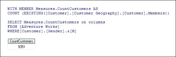
Figure 22 Calculated Measure Using Existing Operator

Summarizing data with MDX

Analysis Services naturally aggregates measures across the attributes of each dimension. While measures provide tremendous analytical value, you may encounter scenarios when you want to perform additional aggregations of data, either aggregating MDX calculations or aggregating subsets of the cube that satisfy specific business rules.

Consider the following examples where you may need to aggregate data in MDX:

  • Performing time series analysis—You need
    to sum reseller profit for all time periods in this year up to and include the current time period.
  • Aggregating custom sets—You need to average year-over-year sales variance across all resellers in the USA who sold more than 10,000 units.
  • Aggregating calculations at dimension leaves—You need to aggregate the hours worked by each employee multiplied by the employee’s hourly rate.

While using MDX calculated measures with functions like Sum, Average, and Aggregate is a valid approach to summarizing data in these scenarios, from a performance perspective, summarizing data through MDX is not a trivial task and can potentially result in slow performance in large-scale cubes or cubes with many nested MDX calculations. If you experience performance issues summarizing data in MDX, you may want to consider the following design alternatives:

Create a named calculation in the data source view

Depending on the scenario, you should first consider whether you need to perform additional aggregations in MDX or whether you can take advantage of the natural aggregation of the cube. Consider the Profit Margin calculation. Profit is defined by Revenue minus Cost. Assuming that these two measures are stored in the same fact table, instead of defining a calculated member that is calculated on the fly, you can move the Profit calculation to a measure. In the data source view you can create a named calculation on the fact table that defines Profit as Revenue minus Cost. Then, you can add the named calculation as a measure in your cube to be aggregated just like every other measure.

Generally speaking, any time that you have a calculated member that performs addition and subtraction from columns on the same fact table, you can move the calculation to measure. If you do this, keep in mind that SQL operations on NULL data are not identical to MDX. In addition, even though you can add the calculation to the fact table, you must also evaluate the impact of additional measures on the cube. Whenever you query a measure group, even if you only request one measure, all measures in that measure group are retrieved from the Storage Engine and loaded into the data cache. The more measures you have, the greater the resource demands. Therefore, it is important to evaluate the performance benefits on a case by case basis.

Use measure expressions

Measure expressions are calculations that the Storage Engine can perform. Using
measure expressions, you can multiply or divide data from two different measure groups at the measure group leaves and then aggregate the data as a part of normal cube processing. The classic example of this is when you have a weighting factor stored in one measure group, such as currency rates, and you want to apply that to another measure group such as sales. Instead of
creating an MDX calculation that aggregates the multiplication of these two measures at the measure group leaves, you can use measure expressions as an optimized solution. This kind of calculation is perfect for a measure expression since it is somewhat more difficult to accomplish in the data source view given that the measures are from different source fact tables and likely have different granularities. To perform the calculation in the data source view, you can use a named query to join the tables; however, the measure expression typically provides a more efficient solution.

While measure expressions can prove to be very useful, note that when you use a measure expression, the Storage Engine evaluates the expression in isolation of the Query Execution Engine. If any of the measures involved in the measure expression depend on MDX calculations, the Storage Engine evaluates the measure expressions without any regard for the MDX calculations, producing an incorrect result set. In this case, rather than using a measure expression, you can use a calculated member or scope assignment.

Use semiadditive measures and unary operators

Instead of writing complex MDX calculations to handle semiadditive measures, you can use the semiadditive aggregate functions like FirstChild, LastChild, etc. Note that semiadditive functions are a feature of SQL Server Enterprise Edition. In addition to using semiadditive measures, in finance applications, instead of writing complicated MDX expressions that apply custom aggregation logic to individual accounts, you can use unary operators with parent-child hierarchies to apply a custom roll up operator for each account. Note that while parent-child hierarchies are restricted in their aggregation design, they can be faster and less complex than custom MDX. For more information on parent-child hierarchies, see Parent-child hierarchies in this white paper.

Move numeric attributes to measures

You can
convert numeric attributes to measures whenever you have an attribute such as Population or Salary that you need to aggregate. Instead of writing MDX expressions to aggregate these values, consider defining a separate measure group on the dimension table containing the attribute and then defining a measure on the attribute column. So for example, you can replace Sum(Customer.City.Members, Customer.Population.MemberValue) by adding a new measure group on the dimension table with a Sum measure on the Population column.

Aggregate subsets of data

In many scenarios, you want to aggregate subsets of data that meet specific business rules. Before you write a complex filter statement to identify the desired set, evaluate whether you can substitute a filter expression by using Crossjoin or Exists with specific members of your attribute hierarchies.

Consider the following examples.

  • If you want a set of resellers with 81 to 100 employees and you have the number of employees stored in a separate attribute, you can easily satisfy this request with the following syntax:

    Exists([Reseller].[Reseller].members,

    [Reseller].[Number of Employees].[81]:

    [Reseller].[Number of Employees].[100])

    In this example, you use Exists with a range for the Number of Employees attribute hierarchy to filter resellers in the 81–100 employee range. The value of this approach is that you can arbitrarily set the ranges based on user requests.

  • If your reseller dimension is large and the ranges that you need to calculate are fixed and commonly used across all users, you can pre-build an attribute that groups the resellers according to employee size ranges. With this new attribute, the previous statement could be written as follows:

    Exists([Reseller].[Reseller].members,

    [Reseller].[Employee Size Range].[81 to 100])

  • Now if you want the sum of the gross profit for resellers with 81 to 100 employees, you can satisfy this request with the following solutions.

    For the range of values, you can use the following syntax.

    Sum([Reseller].[Number of Employees].[81]:

    [Reseller].[Number of Employees].[100],

    [Measures].[Reseller Gross Profit])

    For the custom range attribute, you can use the following syntax.

    ([Reseller].[Number of Employees].[81 – 100],

    [Measures].[Reseller Gross Profit])

    Note that in both of these solutions, the set of resellers is not necessary.

Using an attribute hierarchy to slice data sets provides a superior solution to aggregating a set filtered on member property values, which was a common practice in prior versions of Analysis Services. Retrieving a member’s properties can be slow since each member needs to be retrieved as well as its property value. With attribute hierarchies, you can leverage the normal aggregation of the cube.

Taking advantage of the Query Execution Engine cache

During the execution of an MDX query, the Query Execution Engine stores calculation results in the Query Execution Engine cache. The primary benefits of the cache are to optimize the evaluation of calculations and to support the re-usage of calculation results across users. To understand how the Query Execution Engine uses calculation caching during query execution, consider the following example. You have a calculated member called Profit Margin. When an MDX query requests Profit Margin by Sales Territory, the Query Execution Engine caches the Profit Margin values for each Sales Territory, assuming that the Sales Territory has a nonempty Profit Margin. To manage the re-usage of the cached results across users, the Query Execution Engine uses scopes. Note that Query Execution scopes should not be confused with the SCOPE keyword in an MDX script. Each Query Execution Engine scope maintains its own cache and has the following characteristics.

  • Query
    Scope—The query scope contains any calculations created within a query by using the WITH keyword. The query scope is created on demand and terminates when the query is over. Therefore, the cache of the query scope is not shared across queries in a session.
  • Session
    Scope—The session scope contains calculations created in a given session by using the CREATE statement. The cache of the session scope is reused from request to request in the same session, but is not shared across sessions.
  • Global Scope—The global scope contains the MDX script, unary operators, and custom rollups for a given set of security permissions. The cache of the global scope can be shared across sessions if the sessions share the same security roles.

The scopes are tiered in terms of their level of re-usage. The query scope is considered to be the lowest scope, because it has no potential for re-usage. The global scope is considered to be the highest scope, because it has the greatest potential for re-usage.

During execution, every MDX query must reference all three scopes to identify all of the potential calculations and security conditions that can impact the evaluation of the query. For example, if you have a query that contains a query calculated member, to resolve the query, the Query Execution Engine creates a query scope to resolve the query calculated member, creates a session scope to evaluate session calculations, and creates a global scope to evaluate the MDX script and retrieve the security permissions of the user who submitted the query. Note that these scopes are created only if they aren’t already built. Once they are built for a session, they are usually just re-used for subsequent queries to that cube.

Even though a query references all three scopes, it can only use the cache of a single scope. This means that on a per-query basis, the Query Execution Engine must select which cache to use. The Query Execution Engine always attempts to use the cache of the highest possible scope depending on whether or not the Query Execution Engine detects the presence of calculations at a lower scope.

If the Query Execution Engine detects any calculations that are created at the query scope, it always uses the query scope cache, even if a query references calculations from the global scope. If there are no query-scope calculations, but there are session-scope calculations, the Query Execution Engine uses the cache of session scope. It does not matter whether or not the session calculations are actually used in a query. The Query Execution Engine selects the cache based on the presence of any calculation in the scope. This behavior is especially relevant to users with MDX-generating front-end tools. If the front-end tool creates any session scoped calculations, the global cache is not used, even if you do not specifically use the session calculation in a given query.

There are other calculation scenarios that impact how the Query Execution Engine caches calculations. When you call a stored procedure from an MDX calculation, the engine always uses the query cache. This is because stored procedures are nondeterministic. This means that there is no guarantee of what the stored procedure will return. As a result, nothing will be cached globally or in the session cache. Rather, the calculations will only be stored in the query cache. In addition, the following scenarios determine how the Query Execution Engine caches calculation results:

  • If you enable visual totals for the session by setting the default MDX Visual Mode property of the Analysis Services connection string to 1, the Query Execution Engine uses the query cache for all queries issued in that session.
  • If you enable visual totals for a query by using the MDX VisualTotals function, the Query Execution Engine uses the query cache.
  • Queries that use the subselect syntax (SELECT FROM SELECT) or are based on a session subcube (CREATE SUBCUBE) could cause the query cache to be used.
  • Arbitrary shape sets can only use the query cache when they are used in a subselect, in the WHERE clause, or in a calculated member Aggregate expression referenced in the WHERE clause. An example of arbitrary shape set is a set of multiple members from different levels of a parent-child hierarchy.

Based on this behavior, when your querying workload can benefit from re-using data across users, it is a good practice to define calculations in the global scope. An example of this scenario is a structured reporting workload where you have a few security roles. By contrast, if you have a workload that requires individual data sets for each user, such as in an HR cube where you have a many security roles or you are using dynamic security, the opportunity to re-use calculation results across users is lessened and the performance benefits associated with re-using the Query Execution Engine cache are not as high.

Applying calculation best practices

While many MDX recommendations must be evaluated in the context of a design scenario, the following best practices are optimization techniques that apply to most MDX calculations regardless of the scenario.

Use the Format String property

Instead of applying conditional logic to return customized values if the cell is EMPTY or 0, use the Format String property. The Format String property provides a mechanism to format the value of a cell. You can specify a user-defined formatting expression for positive values, negative values, zeros, and nulls. The Format String display property has considerably less overhead than writing a calculation or assignment that must invoke the Query Execution Engine. Keep in mind that your front-end tool must support this property.

Avoid late-binding functions

When writing MDX calculations against large data sets involving multiple iterations, avoid referencing late binding functions whose metadata cannot be evaluated until run time. Examples of these functions include: LinkMember, StrToSet, StrToMember, StrToValue, and LookupCube. Because they are evaluated at run time, the Query Execution Engine cannot select the most efficient execution path.

Eliminate redundancy

When you use a function that has default arguments such as Time.CurrentMember, you can experience performance benefits if you do not redundantly specify the default argument. For example, use PeriodsToDate([Date].[Calendar].[Calendar Year]) instead of PeriodsToDate([Date].[Calendar].[Calendar Year], [Date].Calendar.CurrentMember). To take advantage of this benefit, you must ensure that you only have one default Time Hierarchy in your application. Otherwise, you must explicitly specify the member in your calculation.

Ordering expression arguments

When writing calculation expressions like “expr1 * expr2”, make sure the expression sweeping the largest area/volume in the cube space and having the most Empty (Null) values is on the left side. For instance, write “Sales * ExchangeRate” instead of “ExchangeRate * Sales”, and “Sales * 1.15” instead of “1.15 * Sales”. This is because the Query Execution Engine iterates the first expression over the second expression. The smaller the area in the second expression, the fewer iterations the Query Execution Engine needs to perform, and the faster the performance.

Use IS

When you need to check the value of a member, use IIF [Customer].[Company] IS [Microsoft] and not IIF [Customer].[Company].Name = “Microsoft”. The reason that IS is faster is because the Query Execution Engine does not need to spend extra time translating members into strings.

Tuning Processing Performance

Processing is the general operation that loads data from one or more data sources into one or more Analysis Services objects. While OLAP systems are not generally judged by how fast they process data, processing performance impacts how quickly new data is available for querying. While every application has different data refresh requirements, ranging from monthly updates to “near real-time” data refreshes, the faster the processing performance, the sooner users can query refreshed data.

Note that “near real-time” data processing is considered to be a special design scenario that has its own set of performance tuning techniques. For more information on this topic, see Near real-time data refreshes.

To help you effectively satisfy your data refresh requirements, the following provides an overview of the processing performance topics that are discussed in this section:

Understanding the processing architecture – For readers unfamiliar with the processing architecture of Analysis Services, this section provides an overview of processing jobs and how they apply to dimensions and partitions. Optimizing processing performance requires understanding how these jobs are created, used, and managed during the refresh of Analysis Services objects.

Refreshing dimensions efficiently – The performance goal of dimension processing is to refresh dimension data in an efficient manner that does not negatively impact the query performance of dependent partitions. The following techniques for accomplishing this goal are discussed in this section: optimizing SQL source queries, reducing attribute overhead, and preparing each dimension attribute to efficiently handle inserts, updates, deletes as necessary.

Refreshing partitions efficiently – The performance goal of partition processing is to refresh fact data and aggregations in an efficient manner that satisfies your overall data refresh requirements. The following techniques for accomplishing this goal are discussed in this section: optimizing SQL source queries, using multiple partitions, effectively handling data inserts, updates, and deletes, and evaluating the usage of rigid vs. flexible aggregations.

Understanding the processing architecture

Processing is typically described in the simple terms of loading data from one or more data sources into one or more Analysis Services objects. While this is generally true, Analysis Services provides the ability to perform a broad range of processing operations to satisfy the data refresh requirements of various server environments and data configurations.

Processing job overview

To manage processing operations, Analysis Services uses centrally controlled jobs. A processing job is a generic unit of work generated by a processing request. Note that while jobs are a core component of the processing architecture, jobs are not only used during processing. For more information on how jobs are used during querying, see Job architecture.

From an architectural perspective, a job can be broken down into parent jobs and child jobs. For a given object, you can have multiple levels of nested jobs depending on where the object is located in the database hierarchy. The number and type of parent and child jobs depend on 1) the object that you are processing such as a dimension, cube, measure group, or partition, and 2) the processing operation that you are requesting such as a ProcessFull, ProcessUpdate, or ProcessIndexes. For example, when you issue a ProcessFull for a measure group, a parent job is created for the measure group with child jobs created for each partition. For each partition, a series of child jobs are spawned to carry out the ProcessFull of the fact data and aggregations. In addition, Analysis Services implements dependencies between jobs. For example, cube jobs are dependent on dimension jobs.

The most significant opportunities to tune performance involve the processing jobs for the core processing objects: dimensions and partitions.

Dimension processing jobs

During the processing of MOLAP dimensions, jobs are used to extract, index, and persist data in a series of dimension stores. For more information on the structure and content of the dimension stores, see Data retrieval: dimensions. To create these dimension stores, the Storage Engine uses the series of jobs displayed in Figure 23.


Figure 23   Dimension processing jobs

Build attribute stores

For each attribute in a dimension, a job is instantiated to extract and persist the attribute members into an attribute store. As stated earlier, the attribute store primarily consists of the key store, name store, and relationship store. While Analysis Services is capable of processing multiple attributes in parallel, it requires that an order of operations must be maintained. The order of operations is determined by the attribute relationships in the dimension. The relationship store defines the attribute’s relationships to other attributes. In order for this store to be built correctly, for a given attribute, all dependent attributes must already be processed before its relationship store is built. To provide the correct workflow, the Storage Engine analyzes the attribute relationships in the dimension, assesses the dependencies among the attributes, and then creates an execution tree that indicates the order in which attributes can be processed, including those attributes that can be processed in parallel.

Figure 24 displays an example execution tree for a Time dimension. The solid arrows represent the attribute relationships in the dimension. The dashed arrows represent the implicit relationship of each attribute to the All attribute. Note that the dimension has been configured using cascading attribute relationships which is a best practice for all dimension designs.


Figure 24   Execution tree example

In this example, the All attribute proceeds first, given that it has no dependencies to another attribute, followed by the Fiscal Year and Calendar Year attributes, which can be processed in parallel. The other attributes proceed according to the dependencies in the execution tree with the primary key attribute always being processed last since it always has at least one attribute relationship, except when it is the only attribute in the dimension.

The time taken to process an attribute is generally dependent on 1) the number of members and 2) the number of attribute relationships. While you cannot control the number of members for a given attribute, you can improve processing performance by using cascading attribute relationships. This is especially critical for the key attribute since it has the most members and all other jobs (hierarchy, decoding, bitmap indexes) are waiting for it to complete. For more information about the importance of using cascading attribute relationships, see Identifying attribute relationships.

Build decoding stores

Decoding stores are used extensively by the Storage Engine. During querying, they are used to retrieve data from the dimension. During processing, they are used to build the dimension’s bitmap indexes.

Build hierarchy stores

A hierarchy store is a persistent representation of the tree structure. For each natural hierarchy in the dimension, a job is instantiated to create the hierarchy stores. For more information on hierarchy stores, see Data retrieval: dimensions.

Build bitmap indexes

To efficiently locate attribute data in the relationship store at querying time, the Storage Engine creates bitmap indexes at processing time. For attributes with a very large number of DataIDs, the bitmap indexes can take some time to process. In most scenarios, the bitmap indexes provide significant querying benefits; however, when you have high cardinality attributes, the querying benefit that the bitmap index provides may not outweigh the processing cost of creating the bitmap index. For more information on this design scenario, see Reducing attribute overhead.

Dimension-processing commands

When you need to perform a process operation on a dimension, you issue dimension processing commands. Each processing command creates one or more jobs to perform the necessary operations.

From a performance perspective, the following dimension processing commands are the most important:

  • A ProcessFull command discards all storage contents of the dimension and rebuilds them. Behind the scenes, ProcessFull executes all dimension processing jobs and performs an implicit ProcessClear to discard the storage contents of all dependent partitions. This means that whenever you perform a ProcessFull of a dimension, you need to perform a ProcessFull on dependent partitions to bring the cube back online.
  • ProcessData discards all storage contents of the dimension and rebuilds only the attribute and hierarchy stores. ProcessData is a component of the ProcessFull operation. ProcessData also clears partitions.
  • ProcessIndexes requires that a dimension already has attribute and hierarchy stores built. ProcessIndexes preserves the data in these stores and then rebuilds the bitmap indexes. ProcessIndexes is a component of the ProcessFull operation.
  • ProcessUpdate does not discard the dimension storage contents, unlike ProcessFull. Rather, it applies updates intelligently in order to preserve dependent partitions. More specifically, ProcessUpdate sends SQL queries to read the entire dimension table and then applies changes to the dimension stores. A ProcessUpdate can handle inserts, updates, and deletions depending on the type of attribute relationships (rigid vs. flexible) in the dimension. Note that ProcessUpdate will drop invalid aggregations and indexes, requiring you to take action to rebuild the aggregations in order to maintain query performance. For more information on applying ProcessUpdate, see Evaluating rigid vs. flexible aggregations.
  • ProcessAdd optimizes ProcessUpdate in scenarios where you only need to insert new members. ProcessAdd does not delete or update existing members. The performance benefit of ProcessAdd is that you can use a different source table or data source view named query that restrict the rows of the source dimension table to only return the new rows. This eliminates the need to read all of the source data. In addition, ProcessAdd also retains flexible aggregations.

For a more comprehensive list of processing commands, see the Analysis Services 2005 Processing Architecture white paper located on the Microsoft Developer Network (MSDN).

Partition-processing jobs

During partition processing, source data is extracted and stored on disk using the series of jobs displayed in Figure 25.


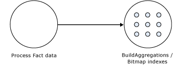
Figure 25   Partition processing jobs

Process fact data

Fact data is processed using three concurrent threads that perform the following tasks:

  • Send SQL statements to extract data from data sources.
  • Look up dimension keys in dimension stores and populate the processing buffer.
  • When the processing buffer is full, write out the buffer to disk.

During the processing of fact data, a potential bottleneck may be the source SQL statement. For techniques to optimize the source SQL statement, see Optimizing the source query.

Build aggregations and bitmap indexes

Aggregations are built in memory during processing. While too few aggregations may have little impact on query performance, excessive aggregations can increase processing time without much added value on query performance. As a result, care must be taken to ensure that your aggregation design supports your required processing window. For more information on deciding which aggregations to build, see Adopting an aggregation design strategy.

If aggregations do not fit in memory, chunks are written to temp files and merged at the end of the process. Bitmap indexes are built on the fact and aggregation data and written to disk on a segment by segment basis.

Partition-processing commands

When you need to perform a process operation on a partition, you issue partition processing commands. Each processing command creates one or more jobs to perform the necessary operations.

From a performance perspective, the following partition processing commands are the most important:

  • ProcessFull discards the storage contents of the partition and rebuilds them. Behind the scenes, a ProcessFull executes ProcessData and ProcessIndexes jobs.
  • ProcessData discards the storage contents of the object and rebuilds only the fact data.
  • ProcessIndexes requires that a partition already has its data built. ProcessIndexes preserves the data and any existing aggregations and bitmap indexes and creates any missing aggregations or bitmap indexes.
  • ProcessAdd internally creates a temporary partition, processes it with the target fact data, and then merges it with the existing partition. Note that ProcessAdd is the name of the XMLA command. This command is exposed in Business Intelligence Development Studio and SQL Server Management Studio as ProcessIncremental.

For a more comprehensive list of processing commands, see Analysis Services 2005 Processing Architecture white paper on MSDN.

Executing processing jobs

To manage dependencies among jobs, the Analysis Services server organizes jobs into a processing schedule. Dimensions, for example, must always be processed first, given the inherent dependency of partitions on dimensions.

Jobs without dependencies can be executed in parallel as long as there are available system resources to carry out the jobs. For example, multiple dimensions can be processed in parallel, multiple measure groups can be processed in parallel, and multiple partitions within a measure group can be processed in parallel. Analysis Services performs as many operations as it can in parallel based on available resources and the values of the following three properties: the CoordinatorExecutionMode server property, and the MaxParallel processing command, and the Threadpool\Process\MaxThreads server property. For more information on these properties, see Maximize parallelism during processing in this white paper.

In addition, before executing a processing job, Analysis Services verifies the available memory. Each job requests a specific amount of memory from the Analysis Services memory governor. If there is not enough memory available to fulfill the memory request, the memory governor can block the job. This behavior can be especially relevant in memory-constrained environments when you issue a processing request that performs multiple intensive operations such as a ProcessFull on a large partition that contains a complex aggregation design. For more information on optimizing this scenario, see Tuning memory for partition processing.

In situations where you are performing querying and processing operations at the same time, a long-running query can block a processing operation and cause it to fail. When you encounter this, the processing operation unexpectedly cancels, returning a generic error message. During the execution of a query, Analysis Services takes a read database commit lock. During processing, Analysis Services requires a write database commit lock. The ForceCommitTimeout server property identifies the amount of time a process operation waits before killing any blocking read locks. Once the timeout threshold has been reached, all transactions holding the lock will fail. The default value for this property is 30,000 milliseconds (30 seconds). Note that this property can be modified in the msmdsrv.ini configuration file; however, it is generally not recommended that you modify this setting. Rather, it is simply important to understand the impact of long-running queries on concurrent processing to help you troubleshoot any unexpected processing failures.

Refreshing dimensions efficiently

As stated previously, the performance goal of dimension processing is to refresh dimension data in an efficient manner that does not negatively impact the query performance of dependent partitions. To accomplish this, you can perform the following techniques: optimize SQL source queries, reduce attribute overhead, and prepare each dimension attribute to efficiently handle inserts, updates, deletes, as necessary.

Optimizing the source query

During processing, you can optimize the extraction of dimension source data using the following techniques:

Use OLE DB Providers over .NET Data Providers

Since the Analysis Services runtime is written in native code, OLE DB Providers offer performance benefits over .NET Data Providers. When you use .NET Data Providers, data has to be marshaled between the .NET managed memory space and the native memory space. Since OLE DB Providers are already in native code, they provide significant performance benefits over.NET Data Providers and should be used whenever possible.

Use attribute relationships to optimize attribute processing across multiple data sources

When a dimension comes from multiple data sources, using cascading attribute relationships allows the system to segment attributes during processing according to data source. If an attribute’s key, name, and attribute relationships come from the same database, the system can optimize the SQL query for that attribute by querying only one database. Without cascading attribute relationships, the SQL Server OPENROWSET function is used to merge the data streams. The OPENROWSET function provides a mechanism to access data from multiple data sources. For each attribute, a separate OPENROWSET-derived table is used. In this situation, the processing for the key attribute is extremely slow since it must access multiple OPENROWSET derived tables.

Tune the Processing Group property

When a dimension is processed, the default behavior is to issue a separate SQL statement that retrieves a distinct set of members for each attribute. This behavior is controlled by the Processing Group property, which is automatically set to ByAttribute. In most scenarios, ByAttribute provides the best processing performance; however, there are a few niche scenarios where it can be useful to change this property to ByTable. In ByTable, Analysis Services issues a single SQL statement on a per-table basis to extract a distinct set of all dimension attributes. This is potentially beneficial in scenarios where you need to process many high cardinality attributes and you are waiting a long time for the select distinct to complete for each attribute. Note that whenever ByTable is used, the server changes its processing behavior to use a multi-pass algorithm. A similar algorithm is also used for very large dimensions when the hash tables of all related attributes do not fit into memory. The algorithm can be very expensive in some scenarios because Analysis Services must read and store to disk all the data from the table in multiple data stores, and then iterate over it for each attribute. Therefore, whatever performance benefit you gain for quickly evaluating the SQL statement could be counteracted by the other processing steps. So while ByTable has the potential to be faster, it is only appropriate in scenarios where you believe that issuing one SQL statement performs significantly better than issuing multiple smaller SQL statements. In addition, note that if you use ByTable, you will see duplicate member messages when processing the dimension if you have configured the KeyDuplicate property to ReportAndContinue or ReportAndStop. In this scenario, these duplicate error messages are false positives resulting from the fact that the SQL statement is no longer returning a distinct set of members for each attribute. To better understand how these duplicates occur, consider the following example. You have a customer dimension table that has three attributes: customer key, customer name, and gender. If you set the Processing Group property to ByTable, one SQL statement is used to extract all three attributes. Given the granularly of the SQL statement, in this scenario, you will see duplicate error messages for the gender attribute if you have set the KeyDuplicate property to raise an error. Again, these error messages are likely false positives; however, you should still examine the messages to ensure that there are no unexpected duplicate values in your data.

Reducing attribute overhead

Every attribute that you include in a dimension impacts the cube size, the dimension size, the aggregation design, and processing performance. Whenever you identify an attribute that will not be used by end users, delete the attribute entirely from your dimension. Once you have removed extraneous attributes, you can apply a series of techniques to optimize the processing of remaining attributes.

Use the KeyColumns and NameColumn properties effectively

When you add a new attribute to a dimension, two properties are used to define the attribute. The KeyColumns property specifies one or more source fields that uniquely identify each instance of the attribute and the NameColumn property specifies the source field that will be displayed to end users. If you do not specify a value for the NameColumn property, it is automatically set to the value of the KeyColumns property.

Analysis Services provides the ability to source the KeyColumns and NameColumn properties from different source columns. This is useful when you have a single entity like a product that is identified by two different attributes: a surrogate key and a descriptive product name. When users want to slice data by products, they may find that the surrogate key lacks business relevance and will choose to use the product name instead.

From a processing perspective, it is a best practice to assign a numeric source field to the KeyColumns property rather than a string property. Not only can this reduce processing time, in some scenarios it can also reduce the size of the dimension. This is especially true for attributes that have a large number of members, i.e., greater than 1 million members.

Rather than using a separate attribute to store a descriptive name, you can use the NameColumn property to display a descriptive field to end users. In the product example, this means you can assign the surrogate key to the KeyColumns property and use the product name to the NameColumn property. This eliminates the need for the extraneous name attribute, making your design more efficient to query and process.

Remove bitmap indexes

During processing of the primary key attribute, bitmap indexes are created for every related attribute. Building the bitmap indexes for the primary key can take time if it has one or more related attributes with high cardinality. At querying time, the bitmap indexes for these attributes are not useful in speeding up retrieval since the Storage Engine still must sift through a large number of distinct values.

For example, the primary key of the customer dimension uniquely identifies each customer by account number; however, users also want to slice and dice data by the customer’s social security number. Each customer account number has a one-to-one relationship with a customer social security number. To avoid spending time building unnecessary bitmap indexes for the social security number attribute, it is possible to disable its bitmap indexes by setting the AttributeHierarchyOptimizedState property to Not Optimized.

Turn off the attribute hierarchy and use member properties

As an alternative to attribute hierarchies, member properties provide a different mechanism to expose dimension information. For a given attribute, member properties are automatically created for every attribute relationship. For the primary key attribute, this means that every attribute that is directly related to the primary key is available as a member property of the primary key attribute.

If you only want to access an attribute as member property, once you verify that the correct relationship is in place, you can disable the attribute’s hierarchy by setting the AttributeHierarchyEnabled property to False. From a processing perspective, disabling the attribute hierarchy can improve performance and decrease cube size because the attribute will no longer be indexed or aggregated. This can be especially useful for high cardinality attributes that have a one-to-one relationship with the primary key. High cardinality attributes such as phone numbers and addresses typically do not require slice-and-dice analysis. By disabling the hierarchies for these attributes and accessing them via member properties, you can save processing time and reduce cube size.

Deciding whether to disable the attribute’s hierarchy requires that you consider both the querying and processing impacts of using member properties. Member properties cannot be placed on a query axis in the same manner as attribute hierarchies and user hierarchies. To query a member property, you must query the properties of the attribute that contains the member property. For example, if you require the work phone number for a customer, you must query the properties of customer. As a convenience, most front-end tools easily display member properties in their user interfaces.

In general, querying member properties can be slower than querying attribute hierarchies because member properties are not indexed and do not participate in aggregations. The actual impact to query performance depends on how you are going to use the attribute. If your users want to slice and dice data by both account number and account description, from a querying perspective you may be better off having the attribute hierarchies in place and removing the bitmap indexes if processing performance is an issue. However, if you are simply displaying the work phone number on a one-off basis for a particular customer and you are spending large amounts of time in processing, disabling the attribute hierarchy and using a member property provides a good alternative.

Optimizing dimension inserts, updates, and deletes

Dimension data refreshes can be generally handled via three processing operations:

  • ProcessFull—Erases and rebuilds the dimension data and structure.
  • ProcessUpdate—Implements inserts, updates, and deletes based on the types of attribute relationships in the dimension. Information on the different types of attribute relationships is included later in this section.
  • ProcessAdd—Provides an optimized version of ProcessUpdate to only handle data insertions.

As you plan a dimension refresh, in addition to selecting a processing operation, you must also assess how each attribute and attribute relationship is expected to change over time. More specifically, every attribute relationship has a Type property that determines how the attribute relationship should respond to data changes. The Type property can either be set to flexible or rigid where flexible is the default setting for every attribute relationship.

Use flexible relationships

Flexible relationships permit you to make a variety of data changes without requiring you to use a ProcessFull to completely rebuild the dimension every time you make a change. Remember that as soon as you implement a ProcessFull on a dimension, the cube is taken offline and you must perform a ProcessFull on every dependent partition in order to restore the ability to query the cube.

For attributes with flexible relationships, inserts, updates, and deletions can be handled by using the ProcessUpdate command. The ProcessUpdate command allows you to keep the cube “online” while the data changes are made. By default, every attribute relationship is set to flexible, although it may not always be the best choice in every design scenario. Using flexible relationships is appropriate whenever you expect an attribute to have frequent data changes and you do not want to experience the impacts of performing a ProcessFull on the dimension and cube. For example, if you expect products to frequently change from one category to another, you may decide to keep the flexible relationship between product and category so that you only need to perform a ProcessUpdate to implement the data change.

The tradeoff to using flexible relationships is their impact on data aggregations. For more information on flexible aggregations, see Evaluating rigid vs. flexible aggregations.

Note that in some processing scenarios, flexible relationships can “hide” invalid data changes in your dimension. As stated in the Identifying attribute relationships section, whenever you use attribute relationships, you must verify that each attribute’s KeyColumns property uniquely identifies each attribute member. If the KeyColumns property does not uniquely identify each member, duplicates encountered during processing are ignored by default, resulting in incorrect data rollups. More specifically, when Analysis Services encounters a duplicate member, it picks an arbitrary member depending on the processing technique that you have selected. If you perform a ProcessFull, it selects the first member it finds. If you perform a ProcessUpdate, it selects the last member it finds. To avoid this scenario, follow the best practice of always assigning the KeyColumns property with a column or combination of columns that unique identifies the attribute. If you follow this practice, you will not encounter this problem. In addition, it is a good practice to change the default error configuration to no longer ignore duplicates. To accomplish this, set the KeyDuplicate property from IgnoreError to ReportAndContinue or ReportAndStop. With this change, you can be alerted of any situation where duplicates are detected. However, this option may give you false positives in some cases (e.g., ByTable processing). For more information, see Optimizing the source query.

Use rigid relationships

For attributes with rigid relationships, inserts can be handled by using a ProcessAdd or ProcessUpdate to the dimension; however, updates and deletions require a ProcessFull of the dimension and consequently require a ProcessFull of the dependent partitions. As such, rigid relationships are most appropriate for attributes that have zero or infrequent updates or deletions. For example, in a time dimension you may assign a rigid relationship between month and quarter since the months that belong to a given quarter do not change.

If you want to assign a relationship as rigid (remember that the relationships are flexible by default), you must ensure that the source data supports the rigid relationship, i.e., no changes can be detected when you perform a ProcessAdd or ProcessUpdate. If Analysis Services detects a change, the dimension process fails and you must perform a ProcessFull. In addition, if you use rigid relationships, duplicate members are never tolerated for a given attribute, unlike in flexible relationships where an arbitrary member is selected during processing. Therefore, you must also ensure that your KeyColumns property is correctly configured.

Similar to flexible relationships, when you define rigid relationships, you must also understand their impact on data aggregations. For more information on rigid aggregations, see Evaluating rigid vs. flexible aggregations.

Refreshing partitions efficiently

The performance goal of partition processing is to refresh fact data and aggregations in an efficient manner that satisfies your overall data refresh requirements. To help you refresh your partitions, the following techniques are discussed in this topic: optimizing SQL source queries, using multiple partitions, effectively handling data inserts, updates, and deletes, and evaluating the usage of rigid vs. flexible aggregations.

Optimizing the source query

To enhance partition processing, there are two general best practices that you can apply for optimizing the source query that extracts fact data from the source database.

Use OLE DB Providers over .NET Data Providers

This is the same recommendation provided for the dimension processing. Since the Analysis Services runtime is written in native code, OLE DB Providers offer performance benefits over.NET Data Providers. When you use .NET Data Providers, data has to be marshaled between the .NET managed memory space and the native memory space. Since OLE DB Providers are already in native code, they provide significant performance benefits over the .NET Data Providers.

Use query bindings for partitions

A partition can be bound to either a source table or a source query. When you bind to a source query, as long as you return the correct number of columns expected in the partition, you can create a wide range of SQL statements to extract source data. Using source query bindings provides greater flexibility than using a named query in the data source view. For example, using query binding, you can point to a different data source using four-part naming and perform additional joins as necessary.

Using partitions to enhance processing performance

In the same manner that using multiple partitions can reduce the amount of data that needs to be scanned during data retrieval (as discussed in How partitions are used in querying), using multiple partitions can enhance processing performance by providing you with the ability to process smaller data components of a measure group in parallel.

Being able to process multiple partitions in parallel is useful in a variety of scenarios; however, there are a few guidelines that you must follow. When you initially create a cube, you must perform a ProcessFull on all measure groups in that cube.

If you process partitions from different client sessions, keep in mind that whenever you process a measure group that has no processed partitions, Analysis Services must initialize the cube structure for that measure group. To do this, it takes an exclusive lock that prevents parallel processing of partitions. If this is the case, you should ensure that you have at least one processed partition per measure group before you begin parallel operations. If you do not have a processed partition, you can perform a ProcessStructure on the cube to build its initial structure and then proceed to process measure group partitions in parallel. In the majority of scenarios, you will not encounter this limitation if you process partitions in the same client session and use the MaxParallel XMLA element to control the level of parallelism. For more information on using MaxParallel, see Maximize parallelism during processing.

After initially loading your cube, multiple partitions are useful when you need to perform targeted data refreshes. Consider the following example. If you have a sales cube with a single partition, every time that you add new data such as a new day’s worth of sales, you must not only refresh the fact data, but you must also refresh the aggregations to reflect the new data totals. This can be costly and time consuming depending on how much data you have in the partition, the aggregation design for the cube, and the type of processing that you perform.

With multiple partitions, you can isolate your data refresh operations to specific partitions. For example, when you need to insert new fact data, an effective technique involves creating a new partition to contain the new data and then performing a ProcessFull on the new partition. Using this technique, you can avoid impacting the other existing partitions. Note that it is possible to use XMLA scripts to automate the creation of a new partition during the refresh of your relational data warehouse.

Optimizing data inserts, updates, and deletes

This section provides guidance on how to efficiently refresh partition data to handle inserts, updates, and deletes.

Inserts

If you have a browseable cube and you need to add new data to an existing measure group partition, you can apply one of the following techniques:

  • ProcessFull—Perform a ProcessFull for the existing partition. During the ProcessFull operation, the cube remains available for browsing with the existing data while a separate set of data files are created to contain the new data. When the processing is complete, the new partition data is available for browsing. Note that a ProcessFull is technically not necessary given that you are only doing inserts. To optimize processing for insert operations, you can use a ProcessAdd.
  • ProcessAdd—Use this operation to append data to the existing partition files. If you frequently perform a ProcessAdd, it is advised that you periodically perform a ProcessFull in order to rebuild and re-compress the partition data files. ProcessAdd internally creates a temp partition and merges it. This results in data fragmentation over time and the need to periodically perform a ProcessFull.

If your measure group contains multiple partitions, as described in the previous section, a more effective approach is to create a new partition that contains the new data and then perform a ProcessFull on that partition. This technique allows you to add new data without impacting the existing partitions. When the new partition has completed processing, it is available for querying.

Updates

When you need to perform data updates, you can perform a ProcessFull. Of course it is useful if you can target the updates to a specific partition so you only have to process a single partition. Rather than directly updating fact data, a better practice is to use a “journaling” mechanism to implement data changes. In this scenario, you turn an update into an insertion that corrects that existing data. With this approach, you can simply continue to add new data to the partition by using a ProcessAdd. You can also have an audit trail of the changes that you have made.

Deletes

For deletions, multiple partitions provide a great mechanism for you to roll out expired data. Consider the following example. You currently have 13 months of data in a measure group, one month per partition. You want to roll out the oldest month from the cube. To do this, you can simply delete the partition without affecting any of the other partitions. If there are any old dimension members that only appeared in the expired month, you can remove these using a ProcessUpdate of the dimension (as long it contains flexible relationships). In order to delete members from the key/granularity attribute of a dimension, you must set the dimension’s UnknownMember property to Hidden or Visible. This is because the server does not know if there is a fact record assigned to the deleted member. With this property set appropriately, it will associate it to the unknown member at query time.

Evaluating rigid vs. flexible aggregations

Flexible and rigid attribute relationships not only impact how you process dimensions, but they also impact how aggregations are refreshed in a partition. Aggregations can either be categorized as rigid or flexible depending on the relationships of the attributes participating in the aggregation. For more information on the impact of rigid and flexible relationships, see Optimizing dimension inserts, updates, and deletes.

Rigid aggregations

An aggregation is rigid when all of the attributes participating in the aggregation have rigid direct or indirect relationships to the granularity attribute of a measure group. For all attributes in the aggregation, a check is performed to verify that all relationships are rigid. If any are flexible, the aggregation is flexible.

Flexible aggregations

An aggregation is flexible when one or more of the attributes participating in the aggregation have flexible direct or indirect relationships to the key attribute.

If you perform a ProcessUpdate on a dimension participating in flexible aggregations, whenever deletions or updates are detected for a given attribute, the aggregations for that attribute as well as any related attributes in the attribute chain are automatically dropped. The aggregations are not automatically recreated unless you perform one of the following tasks:

Note that if you do not follow one of the above techniques, and you perform a ProcessUpdate of a dimension that results in a deletion or update, the flexible aggregations for that attribute and all related attributes in the attribute chain are automatically deleted and not re-created, resulting in poor query performance. This is especially important to note because by default every aggregation is flexible since every attribute relationship type is set to Flexible.

As a result, great care must be taken to ensure that your refresh strategy configures the appropriate attribute relationships for your data changes and effectively rebuilds any flexible aggregations on an ongoing basis.


Optimizing Special Design Scenarios

Throughout this whitepaper, specific techniques and best practices are identified for improving the processing and query performance of Analysis Services OLAP databases. In addition to these techniques, there are specific design scenarios that require special performance tuning practices. Following is an overview of the design scenarios that are addressed in this section:

Special aggregate functions – Special aggregate functions allow you to implement distinct count and semiadditive data summarizations. Given the unique nature of these aggregate functions, special performance tuning techniques are required to ensure that they are implemented in the most efficient manner.

Parent-child hierarchies – Parent-child hierarchies have a different aggregation scheme than attribute and user hierarchies, requiring that you consider their impact on query performance in large-scale dimensions.

Complex Dimension Relationships – Complex dimension relationships include many-to-many relationships and reference relationships. While these relationships allow you to handle a variety of schema designs, complex dimension relationships also require you to assess how the schema complexity is going to impact processing and/or query performance.

Near real-time data refreshes – In some design scenarios, “near real-time” data refreshes are a necessary requirement. Whenever you implement a “near real-time” solution requiring low levels of data latency, you must consider how you are going to balance the required latency with querying and processing performance.

Special aggregate functions

Aggregate functions are the most common mechanism to summarize data. Aggregate functions are uniformly applied across all attributes in a dimension and can be used for additive, semiadditive, and nonadditive measures. Aggregate functions can be categorized into two general groups: traditional aggregate functions and special aggregate functions.

  • Traditional aggregate functions consist of a group of functions that follow the general performance tuning recommendations described in other sections of this white paper. Traditional aggregate functions include Sum, Count, Min, and Max.
  • Special aggregate functions require unique performance-tuning techniques. They include DistinctCount and a collection of semiadditive aggregate functions. The semiadditive functions include: FirstChild, LastChild, FirstNonEmpty, LastNonEmpty, ByAccount, and AverageOfChildren.
Optimizing distinct count

DistinctCount is a nonadditive aggregate function that counts the unique instances of an entity in a measure group. While distinct count is a very powerful analytical tool, it can have significant impact on processing and querying performance because of its explosive impact on aggregation size. When you use a distinct count aggregate function, it increases the size of an aggregation by the number of unique instances that are distinctly counted.

To better understand how distinct count impacts aggregation size, consider the following example. You have a measure group partition with an aggregation that summarizes sales amount by product category and year. You have ten product categories with sales for ten years, producing a total of 100 values in the aggregation. When you add a distinct count of customers to the measure group, the aggregation for the partition changes to include the customer key of each customer who has sales for a specific product category and year. If there are 1,000 customers, the number of potential values in the aggregation increases from 100 to 100,000 values, given that every customer has sales for every product category in every year. (Note that the actual number of values would be less than 100,000 due to natural data sparsity. At any rate, the value is likely to be a number much greater than 100.) While this additional level of detail is necessary to efficiently calculate the distinct count of customers, it introduces significant performance overhead when users request summaries of sales amount by product category and year.

With the explosive impact of distinct counts on aggregations, it is a best practice to separate each distinct count measure into its own measure group with the same dimensionality as the initial measure group. Using this technique, you can isolate the distinct count aggregations and maintain a separate aggregation design for non-distinct count measures.

Note that when you use Business Intelligence Development Studio to create a new measure, if you specify the distinct count aggregate function at the time of the measure creation, the Analysis Services Cube Designer automatically creates a separate measure group for the distinct count measure. However, if you change the aggregate function for an existing measure to distinct count, you must manually reorganize the distinct count measure into its own measure group.

When you are distinctly counting large amount of data, you may find that the aggregations for the distinct count measure group are not providing significant value, since the fact data must typically be queried to calculate the distinct counts. For a distinct count measure group, you should consider partitioning the measure group using data ranges of the distinct count field. For example, if you are performing a distinct count of customers using customer ID, consider partitioning the distinct count measure group by customer ID ranges. In this scenario, partition 1 may contain customer IDs between 1 and 1000. Partition 2 may contain customer IDs between 1001 and 2000. Partition 3 may contain customer IDs between 2001 and 3000, etc. This partitioning scheme improves query parallelism since the server does not have to coordinate data across partitions to satisfy the query.

For larger partitions, to further enhance performance, it may be advantageous to consider an enhanced partitioning strategy where you partition the distinct count measure group by both the distinct count field as well as your normal partitioning attribute, i.e., year, month, etc. As you consider your partitioning strategy for distinct count, keep in mind that when you partition by multiple dimensions, you may quickly find out that you have too many partitions. With too many partitions, in some scenarios you can actually negatively impact query performance if Analysis Services needs to scan and piece together data from multiple partitions at query time. For example, if you partition by sales territory and day, when users want the distinct count of customers by sales territory by year, all of the daily partitions in a specific year must be accessed and assimilated to return the correct value. While this will naturally happen in parallel, it can potentially result in additional querying overhead. To help you determine the size of and scope of your partitions, see the general sizing guidance in the Designing partitions section.

From a processing perspective, whenever you process a partition that contains a distinct count, you will notice an increase in processing time over your other partitions of the same dimensionality. It takes longer to process because of the increased size of the fact data and aggregations. The larger the amount of data that requires processing, the longer it takes to process, and the greater potential that Analysis Services may encounter memory constraints and will need to use temporary files to complete the processing of the aggregation. You must therefore assess whether your aggregation design is providing you with the most beneficial aggregations. To help you determine this, you can use the Usage-Based Optimization Wizard to customize your aggregation design to benefit your query workload. If you want further control over the aggregation design, you may want to consider creating custom aggregations by using the Aggregation Utility described in Appendix C. In addition, you must ensure that the system has enough resources to process the aggregations. For more information on this topic, see Tuning Server Resources.

The other reason that processing time may be slower is due to the fact that an ORDER BY clause is automatically added to the partition’s source SQL statement. To optimize the performance of the ORDER BY in the source SQL statement, you can place a clustered index on the source table column that is being distinctly counted. Keep in mind that this is only applicable in the scenario where you have one distinct count per fact table. If you have multiple distinct counts off of a single fact table, you need to evaluate which distinct count will benefit most from the clustered index. For example, you may choose to apply the clustered index to the most granular distinct count field.

Optimizing semiadditive measures

Semiadditive aggregate functions include ByAccount, AverageOfChildren, FirstChild, LastChild, FirstNonEmpty, and LastNonEmpty. To return the correct data values, semiadditive functions must always retrieve data that includes the granularity attribute of the time dimension. Since semiadditive functions require more detailed data and additional server resources, to enhance performance, semiadditive measures should not be used in a cube that contains ROLAP dimensions or linked dimensions. ROLAP and linked dimensions also require additional querying overhead and server resources. Therefore, the combination of semiadditive measures with ROLAP and/or linked dimensions can result in poor query performance and should be avoided where possible.

Aggregations containing the granularity attribute of the time dimension are extremely beneficial for efficiently satisfying query requests for semiadditive measures. Aggregations containing other time attributes are never used to fulfill the request of a semiadditive measure.

To further explain how aggregations are used to satisfy query requests for semiadditive measures, consider the following example. In an inventory application, when you request a product’s quantity on hand for a given month, the inventory balance for the month is actually the inventory balance for the final day in that month. To return this value, the Storage Engine must access partition data at the day level. If there is an appropriate aggregation that includes the day attribute, the Storage Engine will attempt to use that aggregation to satisfy the query. Otherwise the query must be satisfied by the partition fact data. Aggregations at the month and year cannot be used.

Note that if your cube contains only semiadditive measures, you will never receive performance benefits from aggregations created for nongranularity time attributes. In this scenario, you can influence the aggregation designer to create aggregations only for the granularity attribute of the time dimension (and the All attribute) by setting the Aggregation Usage to None for the nongranularity attributes of the time dimension. Keep in mind that the Aggregation Usage setting automatically applies to all measure groups in the cube, so if the cube contains only semiadditive measures, such as in inventory applications, the Aggregation Usage setting can be uniformly applied across all measure groups.

If you have a mixed combination of semiadditive measures and other measures across measure groups, you can adopt the following technique to apply unique aggregation usage settings to specific measure groups. First, adjust the Aggregation Usage settings for a dimension so that they fit the needs of a particular measure group and then design aggregations for that measure group only. Next, change the Aggregation Usage settings to fit the needs of the next measure group and then design aggregations for that measure group only. Using this approach, you can design aggregations measure group-by-measure group, and even partition-by-partition if desired.

In addition to this technique, you can also optimize the aggregation design using the Usage-Based Optimization Wizard to create only those aggregations that provide the most value for your query patterns. If you want further control over the aggregation design, you may want to consider creating custom aggregations using the Aggregation Utility described in Appendix C.

Parent-child hierarchies

Parent-child hierarchies are hierarchies with a variable number of levels, as determined by a recursive relationship between a child attribute and a parent attribute. Parent-child hierarchies are typically used to represent a financial chart of accounts or an organizational chart. In parent-child hierarchies, aggregations are created only for the key attribute and the top attribute, i.e., the All attribute unless it is disabled. As such, refrain from using parent-child hierarchies that contain large numbers of members at intermediate levels of the hierarchy. Additionally, you should limit the number of parent-child hierarchies in your cube.

If you are in a design scenario with a large parent-child hierarchy (greater than 250,000 members), you may want to consider altering the source schema to re-organize part or all of the hierarchy into a user hierarchy with a fixed number of levels. Once the data has been reorganized into the user hierarchy, you can use the Hide Member If property of each level to hide the redundant or missing members.

Complex dimension relationships

The flexibility of Analysis Services enables you to build cubes from a variety of source schemas. For more complicated schemas, Analysis Services supplies many-to-many relationships and reference relationships to help you model complex associations between your dimension tables and fact tables. While these relationships provide a great deal of flexibility, to use them effectively, you must evaluate their impact on processing and query performance.

Many-to-many relationships

In Analysis Services, many-to-many relationships allow you to easily model complex source schemas. To use many-to-many relationships effectively, you must be familiar with the business scenarios where these relationships are relevant.

Background information on many-to-many relationships

In typical design scenarios, fact tables are joined to dimension tables via many-to-one relationships. More specifically, each fact table record can join to only one dimension table record and each dimension table record can join to multiple fact table records. Using this many-to-one design, you can easily submit queries that aggregate data by any dimension attribute.

Many-to-many design scenarios occur when a fact table record can potentially join to multiple dimension table records. When this situation occurs, it is more difficult to correctly query and aggregate data since the dimension contains multiple instances of a dimension entity and the fact table cannot distinguish among the instances.

To better understand how many-to-many relationships impact data analysis, consider the following example. You have a reseller dimension where the primary key is the individual reseller. To enhance your analysis, you want to add the consumer specialty attribute to the reseller dimension. Upon examining data, you notice that each reseller can have multiple consumer specialties. For example, A Bike Store has two consumer specialties: Bike Enthusiast and Professional Bike. Your sales fact table, however, only tracks sales by reseller, not by reseller and consumer specialty. In other words, the sales data does not distinguish between A Bike Shop with a Bike Enthusiast specialty and A Bike Shop with a Professional Bike specialty. In the absence of some kind of weighting factor to allocate the sales by consumer specialty, it is a common practice to repeat the sales values for each reseller/consumer specialty combination. This approach works just fine when you are viewing data by consumer specialty and reseller; however, it poses a challenge when you want to examine data totals as well as when you want to analyze data by other attributes.

Continuing with the reseller example, if you add the new consumer specialty attribute to the reseller dimension table, whenever the fact table is joined to the dimension table via the individual reseller, the number of records in the result set is multiplied by the number of combinations of reseller and consumer specialty. When the data from this result set is aggregated, it will be inflated. In the example of A Bike Shop, sales data from the fact table will be double-counted regardless of which reseller attribute you group by. This double-counting occurs because A Bike Shop appears twice in the table with two consumer specialties. This data repeating is okay when you are viewing the breakdown of sales by consumer specialty and reseller; however, any sales totals or queries that do not include consumer specialty will be incorrectly inflated.

To avoid incorrectly inflating your data, many-to-many relationships are typically modeled in the source schema using multiple tables as displayed in Figure 26.

  • A main dimension table contains a unique list of primary key values and other attributes that have a one-to-one relationship to the primary key. To enable the dimension table to maintain a one-to-many relationship with the fact table, the multivalued attribute is not included in this dimension. In the reseller example displayed in Figure 26, Dim Reseller is the main dimension table, storing one record per reseller. The multivalued attribute, consumer specialty, is not included in this table.
  • A second dimension table contains a unique list of values for the multivalued attribute. In the reseller example, the Dim Consumer Specialty dimension table stores the distinct list of consumer specialties.
  • An intermediate fact table maps the relationship between the two dimension tables. In the reseller example, Fact Reseller Specialty is an intermediate fact table that tracks the consumer specialties of each reseller.
  • The data fact table stores a foreign key reference to the primary key of the main dimension table. In the reseller example, the Fact Sales table stores the numeric sales data and has a many-to-one relationship with Dim Reseller via the Reseller Key.


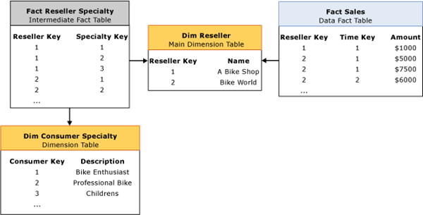
Figure 26   Many-to-many relationship

Using this design, you have maintained the many-to-one relationship between Fact Sales and Dim Reseller. This means that if you ignore Dim Consumer Specialty and Fact Reseller Specialty, you can easily query and aggregate data from Fact Sales by any attribute in the Dim Reseller table without incorrectly inflating values. However this design does not fully solve the problem, since it is still tricky to analyze sales by an attribute in Dim Consumer Specialty. Remember that you still do not have sales broken down by consumer specialty; i.e., sales is only stored by reseller and repeats for each reseller / consumer specialty combination. For queries that summarize sales by consumer specialty, the data totals are still inflated unless you can apply a distinct sum.

To help you accomplish this distinct sum, Analysis Services provides built-in support for many-to-many relationships. Once a many-to-many relationship is defined, Analysis Services can apply distinct sums to correctly aggregate data where necessary. To obtain this benefit in the reseller example, first create the Sales measure group that includes the Dim Reseller dimension and sales measures from the Fact Sales table. Next, you can use a many-to-many relationship to relate the Sales measure group to the Consumer Specialty many-to-many dimension. To set up this relationship, you must identify an intermediate measure group that can be used to map Sales data to Consumer Specialty. In this scenario, the intermediate measure group is Reseller Specialty, sourced from the Fact Reseller Specialty fact table.

Performance considerations

During processing, the data and intermediate measure groups are processed independently. Fact data and aggregations for the data measure group do not include any attributes from the many-to-many dimension. When you query the data measure group by the many-to-many dimension, a run-time “join” is performed between the two measure groups using the granularity attributes of each dimension that the measure groups have in common. In the example in Figure 26, when users want to query Sales data by Consumer Specialty, a run-time join is performed between the Sales measure group and Reseller Specialty measure group using the Reseller Key of the Reseller dimension. From a performance perspective, the run-time join has the greatest impact on query performance. More specifically, if the intermediate measure group is larger than the data measure group or if the many-to-many dimension is generally large (at least one million members), you can experience query performance issues due to the amount of data that needs to be joined at run time. To optimize the run-time join, review the aggregation design for the intermediate measure group to verify that aggregations include attributes from the many-to-many dimension. In the example in Figure 26, aggregations for the intermediate measure group should include attributes from the Consumer Specialty dimension such as the description attribute. While many-to-many relationships are very powerful, to avoid query performance issues, in general you should limit your use of many-to-many relationships to smaller intermediate measure groups and dimensions.

Reference relationships

In traditional dimension design scenarios, all dimension tables join directly to the fact table by means of their primary keys. In snowflake dimension designs, multiple dimension tables are chained together, with the chained dimensions joining indirectly to the fact table by means of a key in another dimension table. These chained dimensions are often called snowflake dimension tables. Figure 27 displays an example of snowflake dimension tables. Each table in the snowflake is linked to a subsequent table via a foreign key reference.


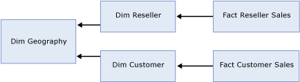
Figure 27   Snowflake dimension tables

In Figure 27, the Dim Reseller table has a snowflake relationship to the Dim Geography table. In addition, the Dim Customer table has a snowflake relationship to the Dim Geography table. From a relational point of view, if you want to analyze customer sales by geography, you must join Dim Geography to Fact Customer Sales via Dim Customer. If you want to analyze reseller sales by geography, you must join Dim Geography to Fact Reseller Sales via Dim Reseller.

Within Analysis Services, dimensions are “joined” to measure groups by specifying the dimension’s relationship type. Most dimensions have regular relationships where a dimension table is joined directly to the fact table. However, for snowflake dimension table scenarios, such as the one depicted in Figure 27, there are two general design techniques that you can adopt as described in this section.

Option 1 – Combine attributes

For each dimension entity that joins to the fact table, create a single OLAP dimension that combines attributes from all of the snowflake dimension tables, and then join each dimension to measure group using a regular relationship type. If you have multiple dimension entities that reference the same snowflake tables, attributes from the shared snowflake tables are repeated across the OLAP dimensions.

To apply this technique to the Figure 27 example, create two OLAP dimensions: 1) a Reseller dimension that contains attributes from both the Dim Reseller and Dim Geography tables, and 2) a Customer dimension that contains attributes from Dim Customer and Dim Geography. Note that attributes from Dim Geography are repeated across both the Reseller and Customer dimensions.

For the Reseller Sales measure group, use a Regular relationship for the Reseller dimension. For the Customer Sales measure group, use a regular relationship Customer dimension. Remember that the relationship between a dimension and a measure group defines how the dimension data is to be “joined” to the fact data. A regular relationship means that you have defined a direct relationship between one or more dimension columns and one or more measure group columns.

With this design, for each OLAP dimension, all of the snowflake dimension tables are joined together at processing time and the OLAP dimension is materialized on disk. As with any other processing operation, you can control whether the processing should remove missing keys or use the unknown member for any records that do join across all tables.

From a performance perspective, the benefit of this approach is the ability to create natural hierarchies and use aggregations. Since each dimension has a regular relationship to the measure group, to enhance query performance, aggregations can be designed for attributes in each dimension, given the proper configuration of attribute relationships. In addition, during querying, you can take advantage of Autoexists optimizations that naturally occur between attributes within a dimension. For more information on Autoexists, see Removing empty tuples.

If you use this approach, you must also consider the impact of increasing the number of attributes that the aggregation design algorithm must consider. By repeating attributes across multiple dimensions, you are creating more work for the aggregation design algorithm which could negatively impact processing times.

Option 2 – Use a reference relationship

An alternative design approach to combining attributes involves reference relationships. Reference relationships allow you to indirectly relate OLAP dimensions to a measure group using an intermediate dimension. The intermediate dimension creates a “join” path that the measure group can use to relate its data to each reference dimension.

To apply this technique to the example in Figure 27, create three separate OLAP dimensions for customer, reseller, and geography. The following describes how these dimensions can be related to each measure group (Reseller Sales and Customer Sales):

  • The Customer Sales measure group contains a regular relationship to the Customer dimension and contains a reference relationship to the Geography dimension. The reference relationship uses Customer as an intermediate dimension to assign sales to specific geographies.
  • The Reseller Sales measure group contains a regular relationship to the Reseller dimension and contains a reference relationship to the Geography dimension. The reference relationship uses Reseller as an intermediate dimension to assign sales to specific geographies.

To use this technique effectively, you must consider the impacts of reference relationships on processing and query performance. During processing, each dimension is processed independently. No attributes from the reference dimension are automatically considered for aggregation. During querying, measure group data is joined to the reference dimension as necessary by means of the intermediate dimension. For example, if you query customer sales data by geography, a run-time join must occur from the Customer Sales measure group to Geography via the Customer dimension. This process can be somewhat slow for large dimensions. In addition, any missing attribute members that are encountered during querying are automatically assigned to the unknown member in order to preserve data totals.

To improve the query performance of reference relationships, you can choose to materialize them. Note that by default, reference relationships are not materialized. When a reference relationship is materialized, the joining across dimensions is performed during processing as opposed to querying. In addition, the attributes in the materialized reference dimensions follow the aggregation rules of standard dimensions. For more information on these rules, see The aggregation usage rules. Since the join is performed during processing and aggregations are possible, materialized reference relationships can significantly improve query performance when compared to unmaterialized relationships.

Some additional considerations apply to materialized reference relationships. During processing, the reference dimension is processed independently. At this time, if any row in the measure group does not join to the reference dimension, the record is removed from the partition. Note that this is different behavior than the unmaterialized reference relationship where missing members are assigned to the unknown member.

To better understand how missing members are handled for materialized relationships, consider the following example. If you have a sales order in the Customer Sales fact table that maps to a specific customer but that customer has a missing geography, the record cannot join to the Geography table and is rejected from the partition. Therefore, if you have referential integrity issues in your source data, materializing the reference relationship can result in missing data from the partition for those fact records that do not join to the reference dimension. To counteract this behavior and handle missing values, you can create your own unknown dimension record in the reference dimension table and then assign that value to all records missing reference values during your extraction, transformation, and loading (ETL) processes. With the unknown record in place for missing values, at processing time, all customer records can successfully join to the reference dimension.

Option Comparison – Combining attributes vs. using reference relationships

When you compare these two design alternatives, it is important to assess the overall impacts on processing and query performance. When you combine attributes, you can benefit from creating natural hierarchies and using aggregations to improve query performance. When you use reference relationships, a reference dimension can only participate in aggregations if it is materialized. These aggregations will not take into account any hierarchies across dimensions, since the reference dimension is analyzed separately from the other dimensions. In light of this information, the following guidelines can help you decide which approach to adopt:

  • If your dimension is frequently queried and can benefit from natural hierarchies and aggregations, you should combine attributes from snowflake dimension tables into your normal dimension design.
  • If the dimension is not frequently queried and is only used for one-off analysis, you can use unmaterialized reference relationships to expose the dimension for browsing without the overhead of creating aggregations for dimension attributes that are not commonly queried. If the intermediate dimensions are large, to optimize the query performance you can materialize the reference relationship.

As an additional design consideration, note that the example in Figure 27 includes snowflake tables with two fact tables / measure groups. When you have snowflake tables that join to a single fact table/ measure group, as depicted in Figure 28, the only available design option is to combine attributes.


Figure 28   One measure group

Reference relationships are not applicable to this design scenario because Analysis Services only allows one reference relationship per dimension per measure group. In the example in Figure 28, this means that when you define Dim Geography as a reference dimension to Reseller Sales, you must either select Dim Reseller or Dim Employee as the intermediate dimension. This either/or selection is not likely going to satisfy your business requirements. As a result, in this scenario, you can use design option 1, combining attributes, to model the snowflake dimension tables.

Near real-time data refreshes

Whenever you have an application that requires a low level of latency, such as in near real-time data refreshes, you must consider a special set of performance tuning techniques that can help you balance low levels of data latency with optimal processing and query performance.

Generally speaking, low levels of data latency include hourly, minute, and second refresh intervals. When you need to access refreshed data on an hourly basis, for example, your first instinct may be to process all of your dimensions and measure groups every hour. However, if it takes 30 minutes to process all database objects, to meet the hourly requirement, you would need to reprocess every 30 minutes. To further complicate this, you would also need to assess the performance impact of any concurrent querying operations that are competing for server resources.

Instead of processing all measure groups and dimensions to meet a low latency requirement, to improve performance and enhance manageability, you can use partitions to isolate the low latency data from the rest of the data. Typically this means that you create one or more near real-time partitions that are constantly being updated with refreshed data. Isolating the low latency data follows normal best practices for partitioning so that you can process and update the near real-time partitions without impacting the other partitions. Using this solution, you can also reduce the amount of data that needs to be processed in near real-time.

With partitions in place, the next step is to decide on how you are going to refresh the data in your near real-time partition(s). Remember that partitions require you to process them in order to refresh the data. Depending on the size of your near real-time partition(s) and the required frequency of the data updates, you can either schedule the refresh of a partition on a periodic basis or you can enable Analysis Services to manage the refresh of a partition using proactive caching.

Proactive caching is a feature in Analysis Services that transparently synchronizes and maintains a partition or dimension much like a cache. A proactive caching partition or dimension is commonly referred to as a cache, even though it is still considered to be a partition or dimension. Using proactive caching, you can enable Analysis Services to automatically detect a data change in the source data, to incrementally update or rebuild the cache with the refreshed data, and to expose the refreshed data to end users.

Even though proactive caching automates much of the refresh work for you, from a performance perspective, you must still consider the typical parameters that impact processing performance such as the frequency of source system updates, the amount of time it takes to update or rebuild the cache, and the level of data latency that end users are willing to accept.

From a performance perspective, there are three groups of settings that impact query responsiveness and processing performance for proactive caching: notification settings, refresh settings, and availability settings.

Notification settings

Notification settings impact how Analysis Services detects data changes in the source system. To satisfy the needs of different data architectures, Analysis Services provides a few mechanisms that you can use to notify Analysis Services of data changes. From a performance perspective, the Scheduled polling mechanism provides the most flexibility by allowing you to either rebuild or incrementally update the cache. Incremental updates improve proactive caching performance by reducing the amount of data that needs to be processed. For proactive caching partitions, incremental updates use a ProcessAdd to append new data to the cache. For proactive caching dimensions, a ProcessUpdate is performed. If you use Scheduled polling without incremental updates, the cache is always completely rebuilt.

Refresh settings

Refresh settings impact when Analysis Services rebuilds or updates the cache. The two most important refresh settings are Silence Interval and Silence Override Interval.

  • Silence Interval defines how long Analysis Services waits from the point at which it detects a change to when it begins refreshing the cache. Since Analysis Services does not officially know when source data changes are finished, the goal is for Analysis Services to refresh the cache when there is a lull in the propagation of source data changes. The lull is defined by a period of silence or no activity that must expire before Analysis Services refreshes the cache. Consider the example where the Silence Interval is set to ten seconds and your cache is configured to be fully rebuilt during refresh. In this scenario, once Analysis Services detects a data change, a time counter starts. If ten seconds pass and no additional changes are detected, Analysis Services rebuilds the cache. If Analysis Services detects additional changes during that time period, the time counter resets each time a change is detected.
  • Silence Override Interval determines how long Analysis Services waits before performing a forced refresh of the cache. Silence Override Interval is useful when your source database is updated frequently and the Silence Interval threshold cannot be reached, since the time counter is continuously reset. In this scenario, you can use the Silence Override Interval to force a refresh of the cache after a certain period of time, such as five minutes or ten minutes. For example, if you set the Silence Override Interval to ten minutes, every ten minutes Analysis Services refreshes the cache only if a change was detected.

Availability settings

Availability settings allow you to control how data is exposed to end users during cache refresh. If
your cache takes several minutes to update or rebuild, you may want to consider configuring the proactive caching settings to allow users to see an older cache until the refreshed cache is ready. For example, if you configure a partition to use Automatic MOLAP settings (Silence Interval = 10 seconds and Silence Override Interval = 10 minutes), during cache refresh, users query the old cache until the new cache is ready. If the cache takes five hours to rebuild, users must wait five hours for cache rebuild to complete. If you always want users to view refreshed data, enable the Bring Online Immediately setting. With Bring Online Immediately enabled, during cache refresh all queries are directed to the relational source database to retrieve the latest data for end users. While this provides users with refreshed data, it can also result in reduced query performance given that Analysis Services needs to redirect queries to the relational source database. If you want finer grained control over users viewing refreshed data, you can use the Latency setting to define a threshold that controls when queries are redirected to the source database during a cache refresh. For example, if you set Latency to four hours and the cache requires five hours to rebuild, for four hours, the queries will be satisfied by the older cache. After four hours, queries are redirected to the source database until the cache has completed its refresh.

Figure 29 illustrates how the proactive caching settings impact queries during cache rebuilding.


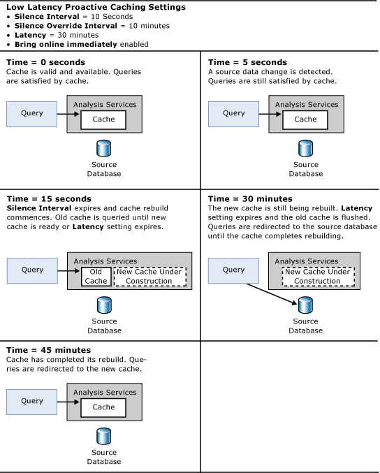
Figure 29   Proactive caching example

Generally speaking, to maximize query performance, it is a good practice to increase Latency where possible so that queries can continue to execute against the existing cache while data is read and processed into a new cache whenever the silence interval or silence override interval is reached. If you set the Latency too low, query performance may suffer as queries are continuously redirected to the relational source. Switching back and forth between the partition and the relational source can provide very unpredictable query response times for users. If you expect queries to constantly be redirected to the source database, to optimize query performance, you must ensure that Analysis Services understands the partition’s data slice. Setting a partition’s data slice is not necessary for traditional partitions. However, the data slice must be manually set for proactive caching partitions, as well as any ROLAP partition. In light of the potential redirection of queries to the relational source, proactive caching is generally not recommended on cubes that are based on multiple data sources.

If you enable proactive caching for your dimensions, to optimize processing, pay special attention to the Latency setting for each dimension and the overall impact of redirecting queries to the source database. When a dimension switches from the dimension cache to the relational database, all partitions that use the dimension need to be fully reprocessed. Therefore, where possible, it is a good idea to ensure that the Latency setting allows you to query the old cache until the new cache is rebuilt.


Tuning Server Resources

Query responsiveness and efficient processing require effective usage of memory, CPU, and disk resources. To control the usage of these resources, Analysis Services 2005 introduces a new memory architecture and threading model that use innovative techniques to manage resource requests during querying and processing operations.

To optimize resource usage across various server environments and workloads, for every Analysis Services instance, Analysis Services exposes a collection of server configuration properties. To provide ease-of-configuration, during installation of Analysis Services 2005, many of these server properties are dynamically assigned based on the server’s physical memory and number of logical processors. Given their dynamic nature, the default values for many of the server properties are sufficient for most Analysis Services deployments. This is different behavior than previous versions of Analysis Services where server properties were typically assigned static values that required direct modification. While the Analysis Services 2005 default values apply to most deployments, there are some implementation scenarios where you may be required to fine tune server properties in order to optimize resource utilization.

Regardless of whether you need to alter the server configuration properties, it is always a best practice to acquaint yourself with how Analysis Services uses memory, CPU, and disk resources so you can evaluate how resources are being utilized in your server environment.

For each resource, this section presents two topics: 1) a topic that describes how Analysis Services uses system resources during querying and processing, and 2) a topic that organizes practical guidance on the design scenarios and data architectures that may require the tuning of additional server properties.

Understanding how Analysis Services uses memory – Making the best performance decisions about memory utilization requires understanding how the Analysis Services server manages memory overall as well as how it handles the memory demands of processing and querying operations.

Optimizing memory usage – Optimizing memory usage requires applying a series of techniques to detect whether you have sufficient memory resources and to identify those configuration properties that impact memory resource utilization and overall performance.

Understanding how Analysis Services uses CPU resources – Making the best performance decisions about CPU utilization requires understanding how the Analysis Services server uses CPU resources overall as well as how it handles the CPU demands of processing and querying operations.

Optimizing CPU usage – Optimizing CPU usage requires applying a series of techniques to detect whether you have sufficient processor resources and to identify those configuration properties that impact CPU resource utilization and overall performance.

Understanding how Analysis Services uses disk resources – Making the best performance decisions about disk resource utilization requires understanding how the Analysis Services server uses disk resources overall as well as how it handles the disk resource demands of processing and querying operations.

Optimizing disk usage – Optimizing disk usage requires applying a series of techniques to detect whether you have sufficient disk resources and to identify those configuration properties that impact disk resource utilization and overall performance.

Understanding how Analysis Services uses memory

Analysis Services 2005 introduces a new memory architecture that allocates and manages memory in a more efficient manner than previous versions of Analysis Services where the memory management of dimensions and other objects placed limits on querying and processing performance. The primary goal of memory management in Analysis Service 2005 is to effectively utilize available memory while balancing the competing demands of processing and querying operations.

To help you gain some familiarity with the distinct memory demands of these two operations, following is a high-level overview of how Analysis Services 2005 uses memory during processing and querying:

  • Querying—During querying, memory is used at various stages of query execution to satisfy query requests. To promote fast data retrieval, the Storage Engine cache is used to store measure group data. To promote fast calculation evaluation, the Query Execution Engine cache is used to store calculation results. To efficiently retrieve dimensions, dimension data is paged into memory as needed by queries, rather than being loaded into memory at server startup, as in prior versions of Analysis Services. To improve query performance, it is essential to have sufficient memory available to cache data results, calculation results, and as-needed dimension data.
  • Processing—During processing, memory is used to temporarily store, index, and aggregate data before writing to disk. Each processing job requests a specific amount of memory from the Analysis Services memory governor. If sufficient memory is not available to perform the job, the job is blocked. To ensure that processing proceeds in an efficient manner, it is important to verify that there is enough memory available to successfully complete all processing jobs and to optimize the calculation of aggregations in memory.

Given the distinct memory demands of querying and processing, it is important to not only understand how each operation impacts memory usage, but it is also important to understand how the Analysis Services server manages memory across all server operations. The sections that follow describe the memory management techniques of the Analysis Services server as well as how it handles the specific demands of querying and processing

Memory management

To effectively understand Analysis Services memory management techniques, you must first consider the maximum amount of memory that Analysis Services can address. Analysis Services relies on Microsoft Windows virtual memory for its memory page pool. The amount of memory it can address depends on the version of SQL Server that you are using:

  • For SQL Server 2005 (32-bit), the maximum amount of virtual memory that an Analysis Services process can address is 3 gigabytes (GB). By default, an Analysis Services process can only address 2 GB; however it is possible to enable Analysis Services to address 3 GB. For guidelines on how to optimize the addressable memory of Analysis Services, see Increasing available memory.
  • SQL Server 2005 (64-bit) is not limited by a 3-GB virtual address space limit, enabling the 64-bit version of Analysis Services to use as much address space as it needs. This applies to both IA64 and X64 architectures.

To perform server operations, Analysis Services requests allocations of memory from the Windows operating system, and then returns that memory to the Windows operating system when the allocated memory is no longer needed. Analysis Services manages the amount of memory allocated to the server by using a memory range that is defined by two server properties: Memory\TotalMemoryLimit and Memory\LowMemoryLimit.

  • Memory\TotalMemoryLimit represents the upper limit of memory that the server uses to manage all Analysis Services operations. If Memory\TotalMemoryLimit is set to a value between 0 and 100, it is interpreted as a percentage of total physical memory. If the property is set to a value above 100, Analysis Services interprets it as an absolute memory value in bytes. The default value for Memory\TotalMemoryLimit is 80, which translates to     80% of the amount of physical memory of the server.
    Note that this property does not define a hard limit on the amount of memory that Analysis Services uses. Rather, it is a soft limit that is used to identify situations where the server is experiencing memory pressure. For some operations, such as processing, if Analysis Services requires additional memory beyond the value of Memory\TotalMemoryLimit, the Analysis Services server attempts to reserve that memory regardless of the value of the property.
  • Memory\LowMemoryLimit represents the lower limit of memory that the server uses to manage all Analysis Services operations. Like the Memory\TotalMemoryLimit property, a value between 0 and 100 is interpreted as a percentage of total physical memory. If the property is set to a value above 100, Analysis Services interprets it as an absolute memory value in bytes.
    The default value for the Memory\LowMemoryLimit property is 75, which translates to 75% of the amount of physical memory on the Analysis Services server.

Analysis Services uses these memory range settings to manage how memory is allocated and used at various levels of memory pressure. When the server experiences elevated levels of memory pressure, Analysis Services uses a set of cleaner threads, one cleaner thread per logical processor, to control the amount of memory allocated to various operations. Depending on the amount of memory pressure, the cleaner threads are activated in parallel to shrink memory as needed. The cleaner threads clean memory according to three general levels of memory pressure:

  • No Memory Pressure—If the memory used by Analysis Services is below the value set in the Memory\LowMemoryLimit property, the cleaner does nothing.
  • Some Memory Pressure—If the memory used by Analysis Services is between the values set in the Memory\LowMemoryLimit and the Memory\TotalMemoryLimit properties, the cleaner begins to clean memory using a cost/benefit algorithm. For more information on how the cleaner shrinks memory, see Shrinkable vs. non-shrinkable memory.
  • High Memory Pressure—If the memory used by Analysis Services is above the value set in the Memory\TotalMemoryLimit property, the cleaner cleans until the memory used by Analysis Services reaches the Memory\TotalMemoryLimit. When the memory used by Analysis Services exceeds the Memory\TotalMemoryLimit, the server goes into an aggressive mode where it cleans everything that it can. If the memory used is mostly non-shrinkable (more information on non-shrinkable memory is included in the next section), and cannot be purged, Analysis Services detects that the cleaner was unable to clean much. If it is in this aggressive mode of cleaning, it tries to cancel active requests. When this point is reached, you may see poor query performance, out of memory errors in the event log, and slow connection times.
Shrinkable vs. non-shrinkable memory

Analysis Services divides memory into two primary categories: shrinkable memory and non-shrinkable memory as displayed in Figure 30.


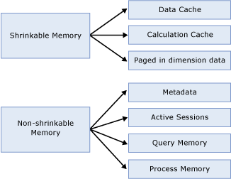
Figure 30   Shrinkable vs. non-shrinkable memory

When the cleaner is activated, it begins evicting elements of shrinkable memory, based on a cost/benefit algorithm that takes into account a variety of factors, including how frequently the entry is used, the amount of resources required to resolve the entries, and how much space is consumed by related entries. Shrinkable memory elements include the following:

  • Cached Results—Cached results include the Storage Engine data cache and Query Execution Engine calculation cache. As stated earlier in this document, the Storage Engine data cache contains measure group data and the Query Execution Calculation Engine cache contains calculation results. While both caches can help improve query response times, the data cache provides the most benefit to query performance by storing data that has been cached from disk. In situations of memory pressure, the cleaner shrinks the memory used for cached results. With this in mind, it is a good practice to monitor the usage of memory so that you can minimize the scenarios where elevated levels of memory pressure force the removal of cached results. For more information on how to monitor memory pressure, see Monitoring memory management.
  • Paged in dimension data—Dimension data is paged in from the dimension stores as needed. The paged-in data is kept in memory until the cleaner is under memory pressure to remove it. Note that this is different behavior than previous versions of Analysis Services where all dimension data was resident in memory.
  • Expired Sessions—Idle client sessions that have exceeded a longevity threshold are removed by the cleaner based on the level of memory pressure. Several server properties work together to manage the longevity of idle sessions. For more information on how to evaluate these properties, see Monitoring the timeout of idle sessions.

Non-shrinkable memory elements are not impacted by the Analysis Services cleaner. Non-shrinkable memory includes the following components:

  • Metadata For each Analysis Services database, metadata is initialized and loaded into memory on demand. Metadata includes the definition of all objects in the database (not the data elements). The more objects in your database (including cubes, measure groups, partitions, and dimensions) and the more databases that you have on a given server, the larger the metadata overhead in memory. Note that this overhead is generally not large for most implementations. However, you can experience significant overhead if your Analysis Services server contains hundreds of databases with tens or hundreds of objects per database, such as in hosted solutions. For more information on how to monitor metadata overheard, see Minimizing metadata overhead.
  • Active Sessions—For each active session, calculated members, named sets, connections, and other associated session information is retained as non-shrinkable memory.
  • Query Memory and Process Memory—Analysis Services reserves specific areas of memory for temporary use during querying and processing. During the execution of a query, for example, memory may be used to materialize data sets such as during the cross joining of data. During processing, memory is used to temporarily store, index, and aggregate data before it are written to disk. These memory elements are non-shrinkable because they are only needed to complete a specific server operation. As soon as the operation is over, these elements are removed from memory.
Memory demands during querying

During querying, memory is primarily used to store cached results in the data and calculation caches. As stated previously, of the two caches, the one that provides the most significant performance benefit is the data cache. When Analysis Services first starts, the data cache is empty. Until the data cache is loaded with data from queries, Analysis Services must resolve user queries by using data stored on disk, either by scanning the fact data or by using aggregations. Once these queries are loaded into the data cache, they remain there until the cleaner thread removes them or the cache is flushed during measure group or partition processing.

You can often increase query responsiveness by preloading data into the data cache by executing a generalized set of representative user queries. This process is called cache warming. While cache warming can be a useful technique, cache warming should not be used as a substitute for designing and calculating an appropriate set of aggregations. For more information on cache warming, see Warming the data cache.

Memory demands during processing

During processing, memory is required to temporarily store fact data and aggregations prior to writing them to disk.

Processing Fact data

Processing uses a double-buffered scheme to read and process fact records from the source database. Analysis Services populates an initial buffer from the relational database, and then populates a second buffer from the initial buffer where the data is sorted, indexed, and written to the partition file in segments. Each segment consists of 65,536 rows; the number of bytes in each segment varies based on the size of each row.

The OLAP\Process\BufferMemoryLimit property controls the amount of memory that is used per processing job to store and cache data coming from a relational data source. This setting along with OLAP\Process\BufferRecordLimit determines the number of rows that can be processed in the buffers. The OLAP\Process\BufferMemoryLimit setting is interpreted as a percentage of total physical memory if the value is less than 100, or an absolute value of bytes if the value is greater than 100. The default value is 60, which indicates that a maximum of 60% of the total physical memory can be used. For most deployments, the default value of OLAP\Process\BufferMemoryLimit provides sufficient processing performance. For more information on scenarios where it may be appropriate to change the value of this property, see Tuning memory for partition processing.

Building Aggregations

Analysis Services uses memory during the building of aggregations. Each partition has its own aggregation buffer space limit. Two properties control the size of the aggregation buffer:

  • OLAP\Process\AggregationMemoryLimitMax is a server property that controls the maximum amount of memory that can be used for aggregation processing per partition processing job. This value is interpreted as a percentage of total memory if the value is less than 100, or an absolute value of bytes if the value is greater than 100. The default value is 80, which indicates that a maximum of 80% of the total physical memory can be used for aggregation processing.
  • OLAP\Process\AggregationMemoryLimitMin is a server property that controls the minimum amount of memory that can be used for aggregation processing per partition processing job. This value is interpreted as a percentage of total memory if the value is less than 100, or an absolute value of bytes if the value is greater than 100. The default value is 10, which indicates that a minimum of 10% of the total physical memory will be used for aggregation processing

For a given partition, all aggregations are calculated at once. As a general best practice, it is a good idea to verify that all aggregations can fit into memory during creation; otherwise temporary files are used, which can slow down processing although the impact on performance is not as significant as in prior versions of Analysis Services. For more information on how to monitor the usage of temporary files, see Tuning memory for partition processing.

Optimizing memory usage

Optimizing memory usage for querying and processing operations requires supplying the server with adequate memory and verifying that the memory management properties are configured properly for your server environment. This section contains a summary of the guidelines that can help you optimize the memory usage of Analysis Services.

Increasing available memory

If you have one or more large or complex cubes and are using SQL Server 2005 (32-bit), use Windows Advanced Server® or Datacenter Server with SQL Server 2005 Enterprise Edition (or SQL Server 2005 Developer Edition) to enable Analysis Services to address up to 3 GB of memory. Otherwise, the maximum amount of memory that Analysis Services can address is 2 GB.

To enable Analysis Services to address more than 2 GB of physical memory with either of these editions, enable the Application Memory Tuning feature of Windows. To accomplish this, use the /3GB switch in the boot.ini file If you set the /3GB switch in the boot.ini file, the server should have at least 4 GB of memory to ensure that the Windows operating system also has sufficient memory for system services. If you run other applications on the server, you must factor in their memory requirements as well.

If you have one or more very large and complex cubes and your Analysis Services memory needs cannot be met within the 3-GB address space, SQL Server 2005 (64-bit) allows the Analysis Services process to access more than 3 GB of memory. You may also want to consider SQL Server 2005 (64-bit) in design scenarios where you have many partitions that you need to process in parallel or large dimensions that require a large amount of memory to process.

If you cannot add additional physical memory to increase performance, increasing the size of the paging files on the Analysis Services server can prevent out–of-memory errors when the amount of virtual memory allocated exceeds the amount of physical memory on the Analysis Services server.

Monitoring memory management

Given that the Memory\TotalMemoryLimit and Memory\LowMemoryLimit
properties are percentages by default, they dynamically reflect the amount of physical memory on the server, even if you add new memory to the server. Using these default percentages is beneficial in deployments where Analysis Services is the only application running on your server.

If Analysis Services is installed in a shared application environment, such as if you have Analysis Services installed on the same machine as SQL Server, consider assigning static values to these properties as opposed to percentages in order to constrain Analysis Services memory usage. In shared application environments, it is also a good idea to constrain how other applications on the server use memory.

When modifying these properties, it is a good practice to keep the difference between the Memory\LowMemoryLimit and Memory\TotalMemoryLimit is at least five percent, so that the cleaner can smoothly transition across different levels of memory pressure.

You can monitor the memory management of the Analysis Services server by using the following performance counters displayed in Table 3.

Table 3   Memory management performance counters

Performance counter name

Definition

MSAS 2005:Memory\Memory Limit Low KB 

Displays the Memory\LowMemoryLimit from the configuration file

MSAS 2005:Memory\Memory Limit High KB 

Displays the Memory\TotalMemoryLimit from the configuration file. 

MSAS 2005:Memory\Memory Usage KB 

Displays the memory usage of the server process. This is the value that is compared to Memory\LowMemoryLimit and Memory\TotalMemoryLimit. Note that the value of this performance counter is the same value displayed by the Process\Private Bytes performance counter.

MSAS 2005:Memory\Cleaner Balance/sec 

Shows how many times the current memory usage is compared against the settings. Memory usage is checked every 500ms, so the counter will trend towards 2 with slight deviations when the system is under high stress.

MSAS 2005:Memory\Cleaner Memory nonshrinkable KB 

Displays the amount of memory, in KB, non subject to purging by the background cleaner.

MSAS 2005:Memory\Cleaner Memory shrinkable KB 

Displays the amount of memory, in KB, subject to purging by the background cleaner. 

MSAS 2005:Memory\Cleaner Memory KB 

Displays the amount of memory, in KB, known to the background cleaner. (Cleaner memory shrinkable + Cleaner memory non-shrinkable.) Note that this counter is calculated from internal accounting information so there may be some small deviation from the memory reported by the operating system.


Minimizing metadata overhead

For each database, metadata is initialized and loaded into non-shrinkable memory. Once loaded into memory, it is not subject to purging by the cleaner thread.

To monitor the metadata overhead for each database

  1. Restart the Analysis Services server.
  2. Note the starting value of the MSAS 2005:Memory\Memory Usage KB performance counter.
  3. Perform an operation that forces metadata initialization of a database, such as iterating over the list of objects in AMO browser sample application, or issuing a backup command on the database.
  4. After the operation has completed, note the ending value of MSAS 2005:Memory\Memory Usage KB. The difference between the starting value and the ending value represents the memory overhead of the database.

For each database, you should see memory growth proportional to the number of databases you initialize. If you notice that a large amount of your server memory is associated with metadata overhead, you may want consider whether you can take steps to reduce the memory overhead of a given database. The best way to do this is to re-examine the design of the cube. An excessive number of dimensions attributes or partitions can increase the metadata overhead. Where possible you should follow the design best practices outlined in Optimizing the dimension design and Reducing attribute overhead.

Monitoring the timeout of idle sessions

Client sessions are managed in memory. In general, there is a one-to-one relationship between connections and sessions. While each connection consumes approximately 32 KB of memory, the amount of memory a given session consumes depends on the queries and calculations performed in that session. You can monitor the current number of user sessions and connections by using the MSAS 2005:Connection\Current
connections and MSAS 2005:Connection\Current
user sessions performance counters to evaluate the connection and session demands on your system.

As stated earlier, active sessions consume non-shrinkable memory, whereas expired sessions consume shrinkable memory. Two main properties determine when a session expires:

  • The MinIdleSessionTimeout is the threshold of idle time in seconds after which the server can destroy a session based on the level of memory pressure. The MinIdleSessionTimeout is set to 2,700 seconds (45 minutes). This means that a session must be idle for 45 minutes before it is considered an expired session that the cleaner can remove when memory pressure thresholds are exceeded.
  • The MaxIdleSessionTimeout is the time in seconds after which the server forcibly destroys an idle session regardless of memory pressure. By default, the MaxIdleSessionTimeout is set to zero seconds, meaning that the idle session is never forcibly removed by this setting.

In addition to the properties that manage expired sessions, there are properties that manage the longevity of sessions that lose their connection. A connectionless session is called an orphaned session.

  • The IdleOrphanSessionTimeout is a server property of that controls the timeout of connection-less sessions. By default this property is set to 120 seconds (three minutes), meaning that if a session loses its connection and a reconnection is not made within 120 seconds, the Analysis Services server forcibly destroys this session.
  • IdleConnectionTimeout controls the timeout of connections that have not been used for a specified amount of time. By default, this property is set to zero seconds. This means that the connection never times out. However, given that the connection cannot exist outside of a session, any idle connection will be cleaned up whenever its session is destroyed.

For most scenarios, these default settings provide adequate server management of sessions. However, there may be scenarios where you want finer-grained session management. For example, you may want to alter these settings according to the level amount of memory pressure that the Analysis Services server is experiencing. During busy periods of elevated memory pressure, you may want to destroy idle sessions after 15 minutes. At times when the server is not busy, you want the idle sessions to be destroyed after 45 minutes. To accomplish this, set the MinIdleSessionTimeout property to 900 seconds (15 minutes) and the MaxIdleSessionTimeout to 2,700 seconds.

Note that before changing these properties, it is important to understand how your client application manages sessions and connections. Some client applications, for example, have their own timeout mechanisms for connections and sessions that are managed independently of Analysis Services.

Tuning memory for partition processing

Tuning memory for partition processing involves three general techniques:

  • Modifying the OLAP\Process\BufferMemoryLimit property as appropriate.
  • Verifying that sufficient memory is available for building aggregations.
  • Splitting up processing jobs in memory-constrained environments.

Modifying the OLAP\Process\BufferMemoryLimit property as appropriate

OLAP\Process\BufferMemoryLimit determines the size of the fact data buffers using during partition processing. While the default value of the OLAP\Process\BufferMemoryLimit is sufficient for many deployments, you may find it useful to alter the property in the following scenarios:

  • If the granularity of your measure group is more summarized than the relational source fact table, generally speaking you may want to consider increasing the size of the buffers to facilitate data grouping. For example, if the source data has a granularity of day and the measure group has a granularity of month, Analysis Services must group the daily data by month before writing to disk. This grouping only occurs within a single buffer and it is flushed to disk once it is full. By increasing the size of the buffer, you decrease the number of times that the buffers are swapped to disk and also decrease the size of the fact data on disk, which can also improve query performance.
  • If the OLAP measure group is of the same granularity as the source relational fact table, you may benefit from using smaller buffers. When the relational fact table and OLAP measure group are at roughly the same level of detail, there is no need to group the data, because all rows remain distinct and cannot be aggregated. In this scenario, assigning smaller buffers is helpful, allowing you to execute more processing jobs in parallel.

Verifying that sufficient memory is available for building aggregations

During processing, the aggregation buffer determines the amount of memory that is available to build aggregations for a given partition. If the aggregation buffer is too small, Analysis Services supplements the aggregation buffer with temporary files. Temporary files are created in the TempDir folder when memory is filled and data is sorted and written to disk. When all necessary files are created, they are merged together to the final destination. Using temporary files can potentially result in some performance degradation during processing; however, the impact is generally not significant given that the operation is simply an external disk sort. Note that this behavior is different than in previous versions of Analysis Services.

To monitor any temporary files used during processing, review the MSAS 2005:Proc Aggregations\Temp file bytes written/sec or the MSAS 2005:Proc Aggregations\Temp file rows written/sec performance counters.

In addition, when processing multiple partitions in parallel or processing an entire cube in a single transaction, you must ensure that the total memory required does not exceed the Memory\TotalMemoryLimit property. If Analysis Services reaches the Memory\TotalMemoryLimit
during processing, it does not allow the aggregation buffer to grow and may cause temporary files to be used during aggregation processing. Furthermore, if you have insufficient virtual address space for these simultaneous operations, you may receive out-of-memory errors. If you have insufficient physical memory, memory paging will occur. If processing in parallel and you have limited resources, consider doing less in parallel.

Splitting up processing jobs in memory-constrained environments

During partition processing in memory-constrained environments, you may encounter a scenario where a ProcessFull operation on a measure group or partition cannot proceed due to limited memory resources. What is happening in this scenario is that the Process job requests an estimated amount of memory to complete the total ProcessFull operation. If the Analysis Services memory governor cannot secure enough memory for the job, the job can either fail or block other jobs as it waits for more memory to become available. As an alternative to performing a ProcessFull, you can split the processing operation into two steps by performing two operations serially: ProcessData and ProcessIndexes. In this scenario, the memory request will be smaller for each sequential operation and is less likely to exceed the limits of the system resources.

Warming the data cache

During querying, memory is primarily used to store cached results in the data and calculation caches. To optimize the benefits of caching, you can often increase query responsiveness by preloading data into the data cache by executing a generalized set of representative user queries. This process is called cache warming. To do this, you can create an application that executes a set of generalized queries to simulate typical user activity in order to expedite the process of populating the query results cache. For example, if you determine that users are querying by month and by product, you can create a set of queries that request data by product and by month. If you run this query whenever you start Analysis Services, or process the measure group or one of its partitions, this will pre-load the query results cache with data used to resolve these queries before users submit these types of query. This technique substantially improves Analysis Services response times to user queries that were anticipated by this set of queries.

To determine a set of generalized queries, you can use the Analysis Services query log to determine the dimension attributes typically queried by user queries. You can use an application, such as a Microsoft Excel macro, or a script file to warm the cache whenever you have performed an operation that flushes the query results cache. For example, this application could be executed automatically at the end of the cube processing step.

Running this application under an identifiable user name enables you to exclude that user name from the Usage-Based Optimization Wizard’s processing and avoid designing aggregations for the queries submitted by the cache warming application.

When testing the effectiveness of different cache-warming queries, you should empty the query results cache between each test to ensure the validity of your testing. You can empty the results cache using a simple XMLA command such as the following:


<Batch
xmlns=http://schemas.microsoft.com/analysisservices/2003/engine>

<ClearCache>

<Object>

<DatabaseID>Adventure Works DW</DatabaseID>

</Object>

</ClearCache>

</Batch>


This example XMLA command clears the cache for the Adventure Works DW database. To execute the ClearCache statement, you can either manually run the XMLA statement in SQL Server Management Studio or use the ASCMD tool command-line utility to execute any XMLA script.


Understanding how Analysis Services uses CPU resources

Analysis Services uses processor resources for both querying and processing. Increasing the number and speed of processors can significantly improve processing performance and, for cubes with a large number of users, improve query responsiveness as well.

Job architecture

Analysis Services uses a centralized job architecture to implement querying and processing operations. A job itself is a generic unit of processing or querying work. A job can have multiple levels of nested child jobs depending on the complexity of the request.

During processing operations, for example, a job is created for the object that you are processing, such as a dimension. A dimension job can then spawn several child jobs that process the attributes in the dimension. During querying, jobs are used to retrieve fact data and aggregations from the partition to satisfy query requests. For example, if you have a query that accesses multiple partitions, a parent job is generated for the query itself along with one or more child jobs per partition.

Generally speaking, executing more jobs in parallel has a positive impact on performance as long as you have enough processor resources to effectively handle the concurrent operations as well as sufficient memory and disk resources. The maximum number of jobs that can execute in parallel across all server operations (including both processing and querying) is determined by the CoordinatorExecutionMode property.

  • A negative value for CoordinatorExecutionMode specifies the maximum number of parallel jobs that can start per processor.
  • A value of zero enables the server to automatically determine the maximum number of parallel operations, based on the workload and available system resources.
  • A positive value specifies an absolute number of parallel jobs that can start per server.

The default value for the CoordinatorExecutionMode is -4, which indicates that four jobs will be started in parallel per processor. This value is sufficient for most server environments. If you want to increase the level of parallelism in your server, you can increase the value of this property either by increasing the number of jobs per processor or by setting the property to an absolute value. While this globally increases the number of jobs that can execute in parallel, CoordinatorExecutionMode is not the only property that influences parallel operations. You must also consider the impact of other global settings such as the MaxThreads server properties that determine the maximum number of querying or processing threads that can execute in parallel. In addition, at a more granular level, for a given processing operation, you can specify the maximum number of processing tasks that can execute in parallel using the MaxParallel command. These settings are discussed in more detail in the sections that follow.

Thread pools

To effectively manage processor resources for both querying and processing operations, Analysis Services 2005 uses two thread pools:

  • Querying thread pool—The querying thread pool controls the worker threads used by the Query Execution Engine to satisfy query requests. One thread from the querying pool is used per concurrent query. The minimum number of threads from the querying pool is determined by the value of the ThreadPool\Query\MinThreads property; its default setting is 1. The maximum number of worker threads maintained in the querying thread pool is determined by the value of ThreadPool\Query\MaxThreads; its default setting is 10.
  • Processing thread pool—The processing thread pool controls the worker threads used by the Storage Engine during processing operations. The processing thread pool is also used during querying to control the threads used by the Storage Engine to retrieve data from disk. The ThreadPool\Process\MinThreads property determines the minimum number of processing threads that can be maintained at a given time. The default value of this property is 1. The ThreadPool\Process\MaxThreads property determines the maximum number of processing threads that can be maintained at a given time. The default value of this property is 64.

For scenarios on when these values should be changed, see Optimizing CPU usage. Before you modify these properties, it is useful to examine how these threads are used during querying and processing.

Processor demands during querying

During querying, to manage client connections, Analysis Services uses a listener thread to broker requests and create new server connections as needed. To satisfy query requests, the listener thread manages worker threads in the querying thread pool and the processing thread pool, assigns worker threads to specific requests, initiates new worker threads if there are not enough active worker threads in a given pool, and terminates idle worker threads as needed.

To satisfy a query request, the thread pools are used as follows:

  • Worker threads from the query pool check the data and calculation caches respectively for any data and/or calculations pertinent to a client request.
  • If necessary, worker threads from the processing pool are allocated to retrieve data from disk.
  • Once data is retrieved, worker threads from the querying pool store the results in the query cache to resolve future queries.
  • Worker threads from the querying pool perform necessary calculations and use a calculation cache to store calculation results.

The more threads that are available to satisfy queries, the more queries that you can execute in parallel. This is especially important in scenarios where you have a large number of users issuing queries. For more information on how to optimize processor resources during querying, see Maximize parallelism during querying.

Processor demands during processing

Where possible, Analysis Services naturally performs all processing operations in parallel. For every processing operation, you can specify the parallelism of the Analysis Services object by using the MaxParallel processing command. By default, the MaxParallel command is configured to Let the server decide, which is interpreted as unlimited parallelism, constrained only by hardware and server workload. For more information on how you can change this setting, see Maximize parallelism during processing.

Of all of the processing operations, partitions place the largest demands on processor resources. Each partition is processed in two stages and each stage is a multithreaded activity.

  • During the first stage of processing a partition, Analysis Services populates an initial buffer from the relational database, populates a second buffer from the initial buffer, and then writes segments to the partition file. Analysis Services utilizes multiple threads for this stage, which execute asynchronously. This means that while data is being added to the initial buffer, data is being moved from the initial buffer into the second buffer and sorted into segments. When a segment is complete, it is written to the partition file. Processor usage during this first phase depends on the speed of the data transfer from the relational tables. Generally this stage is not particularly processor-intensive, using less than one processor. Rather, this stage is generally limited by the speed of retrieving data from the relational database. The maximum size of the buffer used to store the source data is determined by the OLAP\Process\BufferMemoryLimit and OLAP\Process\BufferRecordLimit server
    properties. In some scenarios, it can be beneficial to modify these settings to improve processing performance. For more information on these properties, see Memory demands during processing.
  • During the second stage, Analysis Services creates and computes aggregations for the data. Analysis Services utilizes multiple threads for this stage, executing these tasks asynchronously. These threads read the fact data into an aggregation buffer. If sufficient memory is allocated to the aggregation buffer, these aggregations are calculated entirely in memory. As stated previously in the Memory demands during processing section, if Analysis Services does not have sufficient memory to calculate aggregations, Analysis Services uses temporary files to supplement the aggregation buffer. This stage can be processor-intensive; Analysis Services takes advantage of multiple processors if they are available.
Optimizing CPU usage

While adding additional processor resources can improve the overall performance of Analysis Services, use the following guidelines to optimize the usage of processor resources.

Maximize parallelism during querying

As stated in the Thread pools section, Threadpool\Query\MaxThreads determines the maximum number of worker threads maintained in the querying thread pool. The default value of this property is 10. For servers that have more than one processor, to increase parallelism during querying, consider modifying Threadpool\Query\MaxThreads to be a number dependent on the number of server processors. A general recommendation is to set the Threadpool\Query\MaxThreads to a value of less than or equal to 2 times the number of processors on the server. For example, if you have an eight-processor machine, the general guideline is to set this value to no more than 16. In practical terms, increasing Threadpool\Query\MaxThreads will not significantly increase the performance of a given query. Rather, the benefit of increasing this property is that you can increase the number of queries that can be serviced concurrently.

Since querying also involves retrieving data from partitions, to improve parallel query operations, you must also consider the maximum threads available in the processing pool as specified by the Threadpool\Process\MaxThreads property. By default, this property has a value of 64. While partitions are naturally queried in parallel, when you have many queries that require data from multiple partitions, you can enhance data retrieval by changing the Threadpool\Process\MaxThreads property. When modifying this property, a general recommendation is to set the Threadpool\Process\MaxThreads to a value of less than or equal to 10 times the number of processors on the machine. For example, if you have an eight-processor server, the general guideline is setting this value to no more than 80. Note even though the default value is 64, if you have fewer than eight processors on a given server, you do not need to reduce the default value to throttle parallel operations. As you consider the scenarios for changing the Threadpool\Process\MaxThreads property, remember that changing this setting impacts the processing thread pool for both querying and processing. For more information on how this property specifically impacts processing operations, see Maximizing parallelism during processing.

While modifying the Threadpool\Process\MaxThreads and Threadpool\Query\MaxThreads properties can increase parallelism during querying, you must also take into account the additional impact of the CoordinatorExecutionMode. Consider the following example. If you have a four-processor server and you accept the default CoordinatorExecutionMode setting of
-4, a total of 16 jobs can be executed at one time across all server operations. So if ten queries are executed in parallel and require a total of 20 jobs, only 16 jobs can launch at a given time (assuming that no processing operations are being performed at that time). When the job threshold has been reached, subsequent jobs wait in a queue until a new job can be created. Therefore, if the number of jobs is the bottleneck to the operation, increasing the thread counts may not necessarily improve overall performance.

In practical terms, the balancing of jobs and threads can be tricky. If you want to increase parallelism, it is important to assess your greatest bottleneck to parallelism, such as the number of concurrent jobs and/or the number of concurrent threads, or both. To help you determine this, it is helpful to monitor the following performance counters:

  • MSAS 2005: Threads\Query pool job queue length—The number of jobs in the queue of the query thread pool. A non-zero value means that the number of query jobs has exceeded the number of available query threads. In this scenario, you may consider increasing the number of query threads. However, if CPU utilization is already very high, increasing the number of threads will only add to context switches and degrade performance.
  • MSAS 2005: Threads\Query pool busy threads—The number of busy threads in the query thread pool.


  • MSAS 2005: Threads\Query pool idle threads—The number of idle threads in the query thread pool.
Maximize parallelism during processing

For processing operations, you can use the following mechanisms to maximize parallelism:

  • CoordinatorExecutionMode—As stated earlier, this server-wide property controls the number of parallel operations across the server. If you are performing processing at the same time as querying, it is a good practice to increase this value.
  • Threadpool\Process\MaxThreads—Also discussed earlier in this section, this server-wide property increases the number of threads that can be used to support parallel processing operations.
  • MaxParallel processing command—Rather than globally specifying the number of parallel operations for a given Analysis Services instance, for every processing operation, you can specify the maximum number of tasks that can operate in parallel. In many scenarios, this is the most common setting that is used to affect parallelism. You can specify the MaxParallel command in two ways: the Maximum parallel tasks option in the processing user interface or a custom XMLA script.
    • Maximum parallel tasks option—When you launch a processing operation from SQL Server Management Studio or Business Intelligence Development Studio, you can specify the Maximum parallel tasks option to change the level of parallelism for a given processing operation as displayed in Figure 31. The default value of this setting is Let the server decide,
      which is interpreted as unlimited parallelism, constrained only by hardware and server workload. The drop-down list displays a list of suggested values but you can specify any value. If you increase this value to increase parallelism, be wary of setting the property too high. Performing too many parallel operations at once can be counterproductive if it causes context switching and degrades performance.


      Figure 31   Maximum parallel tasks setting

    • Custom XMLA script —As an alternative to specifying the MaxParallel command in the user interface, you can write a custom XMLA script to perform a processing operation and use the MaxParallel element to control the number of parallel operations within the XMLA script.

When processing multiple partitions in parallel, use the guidelines displayed in Table 4 for the number of partitions that can be processed in parallel according to the number of processors. These guidelines were taken from processing tests performed using Project REAL cubes.

Table 4   Partition processing guidelines


# of Processors 

# of Partitions to be processed in parallel

4 

2 – 4 

8 

4 – 8 

16 

6 – 16


Note that the actual number of partitions that can be processed in parallel depends on the querying workload and design scenario. For example, if you are performing querying and processing at the same time, you may want to decrease the number of partitions processed in parallel in order to keep some free resources for querying. Alternatively, if your design contains SQL queries with many complex joins, your parallel partition processing performance could be limited by the source database. If the source database is on the same machine as Analysis Services, you may see memory and CPU interactions that limit of the benefits of parallel operations. In fact, with too much parallelism you can overload the RDBMS so much that it leads to timeout errors, which cause processing to fail. By default, the maximum number of concurrent connections, and thus queries, for a data source is limited to ten. This can be changed by altering the Maximum Number of Connections setting of the data source properties in either Business Intelligence Development Studio or SQL Server Management Studio.

To help you monitor the number of partitions processing in parallel, you can review the MSAS 2005:Processing\Rows read/sec performance counter. Generally you should expect this counter to display 40,000–60,000 rows per second for one partition. If your partition contains complex SQL joins or hundreds of source columns, you are likely to see a lower rate. Additionally, you can monitor the number of threads being used during processing by using the MSAS 2005: Threads\Processing pool busy threads performance counter. You can also view jobs that are waiting to execute by using the MSAS 2005: Threads\Processing pool job queue length performance counter.

Note that when you perform parallel processing of any object, all parallel operations are committed in one transaction. In other words, it is not possible to perform a parallel execution and then commit each transaction as it progresses. While this is not specifically a performance issue, it does impact your processing progress. If you encounter any errors during processing, the entire transaction rolls back.

Use sufficient memory

The Optimizing memory usage section describes techniques to ensure that Analysis Services has sufficient memory to perform querying and processing operations. Ensuring that Analysis Services has sufficient memory can also impact Analysis Services usage of processor resources. If the Analysis Services server has sufficient memory, the Windows operating system will not need to page memory from disk. Paging reduces processing performance and query responsiveness. 

Use a load-balancing cluster

If your performance bottleneck is processor utilization on a single system as a result of a multi-user query workload, you can increase query performance by using a cluster of Analysis Services servers to service query requests. Requests can be load balanced across two Analysis Services servers, or across a larger number of Analysis Services servers to support a large number of concurrent users (this is called a server farm). Load-balancing clusters generally scale linearly. Both Microsoft and third-party vendors provide cluster solutions. The Microsoft load-balancing solution is Network Load Balancing (NLB), which is a feature of the Windows Server operating system. With NLB, you can create an NLB cluster of Analysis Services servers running in multiple host mode. When an NLB cluster of Analysis Services servers is running in multiple host mode, incoming requests are load balanced among the Analysis Services servers. When you use a load-balancing cluster, be aware that the data caches on each of the servers in the load-balancing cluster will be different, resulting in differences in query response times from query to query by the same client.

A load-balancing cluster can also be used to ensure availability in the event that a single Analysis Services server fails. An additional option for increasing performance with a load-balancing cluster is to distribute processing tasks to an offline server. When new data has been processed on the offline server, you can update the Analysis Services servers in the load-balancing cluster by using Analysis Services database synchronization.

If your users submit a lot of queries that require fact data scans, a load-balancing cluster may be a good solution. For example, queries that may require a large number of fact data scans include wide queries (such as top count or medians), and random queries against very complex cubes where the probability of hitting an aggregation is very low.

However, a load-balancing cluster is generally not needed to increase Analysis Services performance if aggregations are being used to resolve most queries. In other words, concentrate on good aggregation and partitioning design first. In addition, a load-balancing cluster does not solve your performance problem if processing is the bottleneck or if you are trying to improve an individual query from a single user. Note that one restriction to using a load-balancing cluster is the inability to use writeback, because there is no single server to which to write back the data.

Understanding how Analysis Services uses disk resources

Analysis Services uses disk I/O resources for both querying and processing. Increasing the speed of your disks, spreading the I/O across multiple disks, and using multiple controllers, can significantly improve processing performance. These steps also significantly improve query responsiveness when Analysis Services is required to perform fact data scans. If you have a large number of queries that require fact data scans, Analysis Services can become constrained by insufficient disk I/O when there is not enough memory to support the file system cache in addition to Analysis Services memory usage.

Disk resource demands during processing

As stated previously in the Memory demands during processing section, during processing, the aggregation buffer determines the amount of memory that is available to build aggregations for a given partition. If the aggregation buffer is too small, Analysis Services uses temporary files. Temporary files are created in the TempDir folder when memory is filled and data is sorted and written to disk. When all necessary files are created, they are merged together to the final destination. Using temporary files can result in some performance degradation during processing; however, the impact is generally not significant given that the operation is simply an external disk sort. Note that this behavior is different than previous versions of Analysis Services. To monitor any temporary files used during processing, review the MSAS 2005:Proc Aggregations\Temp file bytes written/sec or the MSAS 2005:Proc Aggregations\Temp file rows written/sec performance counters.

Disk resource demands during querying

During querying, Analysis Services may request arbitrary parts of the data set, depending on user query patterns. When scanning a single partition, the I/Os are essentially sequential, except that large chunks may be skipped because the indexes may indicate that they aren’t needed. If commonly used portions of the cube (particularly the mapping files) fit in the file system cache, the Windows operating system may satisfy the I/O requests from memory rather than generating physical I/O. With large cubes, using a 64-bit version of the Microsoft Windows Server 2003 family increases the amount of memory that the operating system can use to cache Analysis Services requests. With sufficient memory, much of the cube can be stored in the file system cache.

Optimizing disk usage

While increasing disk I/O capacity can significantly improve the overall performance of Analysis Services, there are several steps you can take to use existing disk I/O more effectively. This section contains guidelines to help you optimize disk usage of Analysis Services.

Using sufficient memory

The Optimizing memory usage section describes techniques to ensure that Analysis Services has sufficient memory to perform querying and processing operations. Ensuring that Analysis Services has sufficient memory can also impact Analysis Services usage of disk resources. For example, if there is not enough memory to complete processing operations, Analysis Services uses temporary files, generating disk I/O.

If you cannot add sufficient physical memory to avoid memory paging, consider creating multiple paging files on different drives to spread disk I/O across multiple drives when memory paging is required.

Optimizing file locations

The following techniques can help you to optimize the data files and temporary files used during processing:

•    Place the Analysis Services data files on a fast disk subsystem.

The location of the data files is determined by the DataDir server property. To optimize disk access for querying and processing, place the Analysis Services Data folder on a dedicated disk subsystem (RAID 5, RAID 1+0, or RAID 0+1).

•    If temporary files are used during processing, optimize temporary file disk I/O.

The default location of the temporary files created during aggregation processing is controlled by the TempDir property. If a temporary file is used, you can increase processing performance by placing this temporary folder on a fast disk subsystem (such as RAID 0 or RAID 1+0) that is separate from the data disk.

Disabling unnecessary logging

Flight Recorder provides a mechanism to record Analysis Services server activity into a short-term log. Flight Recorder provides a great deal of benefit when you are trying to troubleshoot specific querying and processing problems; however, it introduces a certain amount of I/O overheard. If you are in a production environment and you do not require Flight Recorder capabilities, you can disable its logging and remove the I/O overhead. The server property that controls whether Flight Recorder is enabled is the Log\Flight Recorder\Enabled property. By default, this property is set to true.


Conclusion

For more information:

http://www.microsoft.com/technet/prodtechnol/sql/2005/technologies/ssasvcs.mspx


Did this paper help you? Please give us your feedback. On a scale of 1 (poor) to 5 (excellent), how would you rate this paper?


Appendix A – For More Information

The following white papers might be of interest.


Appendix B – Partition Storage Modes

Each Analysis Services partition can be assigned a different storage mode that specifies where fact data and aggregations are stored. This appendix describes the various storage modes that Analysis Services provides: multidimensional OLAP (termed MOLAP), hybrid OLAP (HOLAP), and relational OLAP (ROLAP). Generally speaking. MOLAP provides the fastest query performance; however, it typically involves some degree of data latency.

In scenarios where you require near real-time data refreshes and the superior query performance of MOLAP, Analysis Services provides proactive caching. Proactive caching is an advanced feature that requires a special set of performance tuning techniques to ensure that it is applied effectively. For more information on the performance considerations of using proactive caching, see Near real-time data refreshes in this white paper.

Multidimensional OLAP (MOLAP)

MOLAP partitions store aggregations and a copy of the source data (fact and dimension data) in a multidimensional structure on the Analysis Services server. All partitions are stored on the Analysis Services server.

Analysis Services responds to queries faster with MOLAP than with any other storage mode for the following reasons:

  • Compression—Analysis Services compresses the source fact data and its aggregations to approximately 30 percent of the size of the same data stored in a relational database. The actual compression ratio varies based on a variety of factors, such as the number of duplicate keys and bit encoding algorithms. This reduction in storage size enables Analysis Services to resolve a query against fact data or aggregations stored in a MOLAP structure much faster than against data and aggregations stored in a relational structure because the size of the physical data being retrieved from the hard disk is smaller.
  • Multidimensional data structures—Analysis Services uses native multidimensional data structures to quickly find the fact data or aggregations. With ROLAP and HOLAP partitions, Analysis Services relies on the relational engine to perform potentially large table joins against fact data stored in the relational database to resolve some or all queries. Large table joins against relational structures take longer to resolve than similar queries against the MOLAP structures.
  • Data in a single service—MOLAP partitions are generally stored on a single Analysis Services server, with the relational database frequently stored on a server separate from the Analysis Services server. When the relational database is stored on a separate server and partitions are stored using ROLAP or HOLAP, Analysis Services must query across the network whenever it needs to access the relational tables to resolve a query. The impact of querying across the network depends on the performance characteristics of the network itself. Even when the relational database is placed on the same server as Analysis Services, inter-process calls and the associated context switching are required to retrieve relational data. With a MOLAP partition, calls to the relational database, whether local or over the network, do not occur during querying.
Hybrid OLAP (HOLAP)

HOLAP partitions store aggregations in a multidimensional structure on the Analysis Services server, but leave fact data in the original relational database. As a result, whenever Analysis Services needs to resolve a query against fact data stored in a HOLAP partition, Analysis Services must query the relational database directly rather than querying a multidimensional structure stored on the Analysis Services server. Furthermore, Analysis Services must rely on the relational engine to execute these queries. Querying the relational database is slower than querying a MOLAP partition because of the large table joins generally required.

Some administrators choose HOLAP because HOLAP appears to require less total storage space while yielding excellent query performance for many queries. However, these apparent justifications for using HOLAP storage option are negated by the likelihood of excessive aggregations and additional indexes on relational tables.

  • Excessive aggregations—Query responsiveness with HOLAP partitions relies on the existence of appropriate aggregations so that Analysis Services does not have to resolve queries against the fact table in the relational database. To ensure that a wide range of aggregations exists, administrators sometimes resort to generating excessive aggregations by increasing the performance improvement percentage in the Aggregation Design Wizard, or artificially increasing the partition row counts (and sometimes both). While these techniques increase the percentage of queries that Analysis Services can resolve using aggregations, there will always be some queries that can only be resolved against the fact data (remember the one-third rule). In addition, generating additional aggregations to improve query responsiveness comes at the cost of significantly longer processing times and increased storage requirements (which also negates the space savings).
  • Additional indexes on relational tables—To ensure that the relational engine can quickly resolve queries that Analysis Services must resolve against the fact table in the relational database, administrators often add appropriate indexes to the fact and dimension tables. These additional indexes frequently require more space than MOLAP requires to store the entire cube. The addition of these indexes negates the apparent savings in disk space that is sometimes used to justify HOLAP. In addition, maintaining the indexes on the relational tables slows the relational engine when adding new data to the relational tables.

From a processing perspective, there is no significant difference in processing performance between MOLAP partitions and HOLAP partitions. In both cases, all fact data is read from the relational database, and aggregations are calculated. With MOLAP, Analysis Services writes the fact data into the MOLAP structure. With HOLAP, Analysis Services does not store fact data. This difference has minimal impact on processing performance, but can have a significant impact on query performance. Because HOLAP and MOLAP processing speeds are approximately the same and MOLAP query performance is superior, MOLAP is the optimum storage choice.

Relational OLAP (ROLAP)

ROLAP partitions store aggregations in the same relational database that stores the fact data. By default, ROLAP partitions store dimensions in MOLAP on the Analysis Services server, although the dimensions can also be stored using ROLAP in the relational database (for very large dimensions). Analysis Services must rely on the relational engine to resolve all queries against the relational tables, storing both fact data and aggregations. The sheer number of queries with large table joins in large or complex cubes frequently overwhelms the relational engine.

Given the slower query performance of ROLAP, the only situation in which ROLAP storage should be used is when you require reduced data latency and you cannot use proactive caching. For more information on proactive caching, see Near real-time data refreshes in this white paper. In this case, to minimize the performance cost with ROLAP, consider creating a small near real-time ROLAP partition and create all other partitions using MOLAP. Using MOLAP for the majority of the partitions in a near real-time OLAP solution allows you to optimize the query responsiveness of Analysis Services for most queries, while obtaining the benefits of real-time OLAP.

From a processing perspective, Analysis Services can store data, create MOLAP files, and calculate aggregations faster than a relational engine can create indexes and calculate aggregations. The primary reason the relational engine is slower is due to the large table joins that the relational engine must perform during the processing of a ROLAP partition. In addition, because the relational engine performs the actual processing tasks, competing demands for resources on the computer hosting the relational tables can negatively affect processing performance for a ROLAP partition.

Appendix C – Aggregation Utility

As a part of the Analysis Services 2005 Service Pack 2 samples, the Aggregation Utility is an advanced tool that complements the Aggregation Design Wizard and the Usage-Based Optimization Wizard by allowing you to create custom aggregation designs without using the aggregation design algorithm. This is useful in scenarios where you need to override the algorithm and create a specific set of aggregations to tune your query workload. Rather than relying on the cost/benefit analysis performed by the algorithm, you must decide which aggregations are going to be most effective to improve query performance without negatively impacting processing times.

Benefits of the Aggregation Utility

The Aggregation Utility enables you to complete the following tasks.

View and modify specific aggregations in an existing aggregation design.

Using the Aggregation Utility, you can view, add, delete, and change individual aggregations in existing designs. Once you build an aggregation design using the Aggregation Design Wizard or Usage-Based Optimization Wizard, you can use the utility to view the attributes that make up each aggregation. In addition, you have the ability to modify an individual aggregation by changing the attributes that participate in the aggregation.

Create new aggregation designs.

You can either create new aggregation designs by manually selecting the attributes for the aggregations, or by using the utility to build aggregations based on the query log. Note that the Aggregation Utility’s ability to build aggregations from the query log is very different than the functionality of the Usage-Based Optimization Wizard. Remember that the Usage-Based Optimization Wizard reads data from the query log and then uses the aggregation design algorithm to determine whether or not an aggregation should be built. While the Usage-Based Optimization Wizard gives greater consideration to the attributes contained in the query log, there is no absolute guarantee that they will be built.

When you use the Aggregation Utility to build new aggregations from the query log, you decide which aggregations provide the most benefit for your query performance without negatively impacting processing times. In other words, you are no longer relying on the aggregation design algorithm to select which aggregations are built. To help you make effective decisions, the utility enables you to optimize your design, including the ability to remove redundancy, eliminate duplicates, and remove large aggregations that are close to the size of the fact table.

Review whether aggregations are flexible or rigid.

A bonus of the Aggregation Utility is the ability to easily identify whether an aggregation is flexible or rigid. By default, aggregations are flexible. Remember that in a flexible aggregation, one or more attributes have flexible relationships while in a rigid aggregation, all attributes have rigid relationships. If you want change an aggregation from flexible to rigid, you must first change all of the necessary attribute relationships. Once you make these changes, you can use the utility to confirm that you have been successful as the aggregation will now be identified as rigid. Without the utility, you need to manually review the aggregation files in the operating system to determine whether they were flexible or rigid. For more information on rigid and flexible aggregations, see Evaluating rigid vs. flexible aggregations in this white paper.

How the Aggregation Utility organizes partitions

Using the Aggregation Utility, you can connect to an instance of Analysis Services and manage aggregation designs across all of the cubes and databases in that instance. For each measure group, the Aggregation Utility groups partitions by their aggregation designs. Figure 32 displays an example of this grouping.


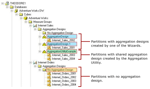
Figure 32   Aggregation display for the Internet Sales measure group

The partitions in Figure 32 are grouped as follows:

  • Aggregation design created by a wizard—Aggregation designs created by the Aggregation Design Wizard or the Usage-Based Optimization Wizard are automatically named AggregationDesign, with an optional number suffix if more than one Wizard-created aggregation design exists per measure group. For example, in the Internet Sales measure group, the Internet_Sales_2002 partition has an aggregation design named AggregationDesign, and the Internet_Sales_2001 partition contains an aggregation design named AggregationDesign 1. Both AggregationDesign and AggregationDesign 1 were created by one of the wizards.
  • Aggregation design created by the Aggregation Utility—The Internet_Sales_2003 and Internet_Sales_2004 partitions share an aggregation design, called AggregationUtilityExample. This aggregation design was created by the Aggregation Utility. The Aggregation Utility allows you to provide a custom name for each aggregation design.
  • No Aggregation Design—For the Internet Orders measure group, none of the partitions in that measure group have an aggregation design yet.
How the Aggregation Utility works

The most common scenario for using the Aggregation Utility is to design aggregations based on a query log. Following is a list of steps to effectively use the Aggregation Utility to design new aggregations based on the query log.

To add new aggregations based on the query log

  1. Perform pre-requisite set up tasks.

    Before using the Aggregation Utility, you must configure Analysis Services query logging just as you would before you use the Usage-Based Optimization Wizard. As you set up query logging, pay close attention to configure an appropriate value for the QueryLogSampling property. The default value of this property is set to one out of every ten queries. Depending on your query workload, you may need to increase this value in order to collect a representative set of queries in the Analysis Services query log table. Obtaining a good sampling of queries is critical to effectively using the Aggregation Utility.

  2. Add a new aggregation design based on a query log.

    To extract data from the query log table, the Aggregation Utility provides a default query that returns a distinct list of datasets for a given partition. A dataset is the subcube that is used to satisfy query requests. An example of the default query is depicted in the query below. The values highlighted in yellow are placeholder values.


Select distinct dataset from OLAPQueryLog

Where MSOLAP_Database = DatabaseName and

MSOLAP_ObjectPath = MeasureGroupName


Generally speaking, it is a good idea to modify the default SQL statement to apply additional filters that restrict the records based on Duration or MSOLAP_User. For example, you may only return queries where the Duration > 30 seconds or MSOLAP_User = Joe.

In addition, whenever you add a new aggregation design by using the Aggregation Utility, it is a good idea to use a special naming convention to name the aggregation design as well as the aggregation prefix. This allows you to easily identify those aggregations that have been created by the utility. For example, when you use SQL Server Profiler to analyze the effectiveness of your aggregations, with easily recognizable names, you will be able to quickly identify those aggregations that have been created by the Aggregation Utility.

  1. Eliminate redundant aggregations.

    You can optimize a new aggregation design by eliminating redundant aggregations. Redundant aggregations are those aggregations that include one or more attributes in the same attribute relationship tree.

    The aggregation highlighted in Figure 33 identifies an aggregation with attributes from two dimensions: Product and Time. From the product dimension, the aggregation includes the English Product Category Name
    attribute. From the Time dimension, the aggregation includes the following attributes: English Month Name, Calendar Quarter, and Calendar Year. This is a redundant aggregation since English Month Name, Calendar Quarter, and Calendar Year are in the same attribute relationship tree.


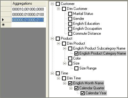
    Figure 33   Redundant aggregation example

    To remove the redundancy in this aggregation, use the Eliminate Redundancy option in the Aggregation Utility. Figure 34 displays the aggregation after the Eliminate Redundancy option is applied. The aggregation now only includes the English Month Name attribute from the Time dimension.


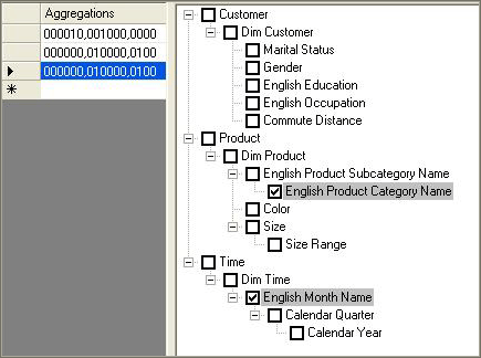
    Figure 34   Aggregations with redundancy eliminated


  1. Eliminate duplicate aggregations.

    Duplicate aggregations are aggregations that include the exact same set of attributes. Continuing with example in Figure 34, note that the there are two identical aggregations for 0000000,010000,0100. This aggregation consists of the English Product Category
    Name and English Month Name attributes. After the Eliminate Duplicates option is applied, the duplicated aggregation is removed and the updated aggregation design is presented in Figure 35.


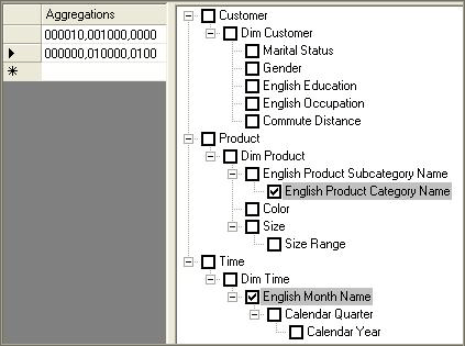
    Figure 35   Aggregations with duplicates eliminated


  1. Assign the aggregation design to a partition.

    After you assign the aggregation design to one or more partitions, the utility displays the assigned partitions under the name of the new aggregation design, as displayed in Figure 32.

  2. Save the measure group to SQL Server.

    Your new aggregation design and partition assignment is not saved on the server until you perform an explicit save on the modified measure group. If you exit out of the utility and do not save, your changes will not be committed to the server.

  3. Process the
    partition.

    Process the necessary measure group or partitions to build the aggregations for your new design. This operation needs to be performed outside of the Aggregation Utility using your normal processing techniques. Note that if you simply need to build aggregations, you can perform a ProcessIndexes operation on the appropriate measure group / partitions. For more information on ProcessIndexes, see Partition-processing commands.

  4. Evaluate
    the
    aggregation size.

    With the aggregations processed, you can use the Aggregation Utility to evaluate the relative size of each aggregation compared with the fact data for the partition. Using this information, you manually eliminate relatively large aggregations that take a long time to process and do not offer significant querying benefits. Remember that the aggregation design algorithm eliminates any aggregations that are greater than one third the size of the fact table. To apply similar logic, you can easily identify and delete any aggregations in your custom aggregation design that are significantly large.

  5. Re-save to SQL Server and reprocess.

    After you evaluate the aggregation size and remove any large aggregations, re-save the aggregation design and then reprocess the necessary partitions. For any subsequent changes that you make over time, always remember to re-save and reprocess.

UPGRADING FARMS FROM SHAREPOINT 2007 TO SP2010

INTRODUCTION ………………………………………………………………………………………………………….. 4 1.1. Outline ……………………………………………………………………………………………………………………… 4 1.2. Acknowledgements ………………………………………………………………………………………………….. 4 1.3. Updates ……………………………………………………………………………………………………………………. 4 2. UPGRADING FARMS FROM SHAREPOINT 2007 TO SP2010 ……………………………………………….. 5 2.1. The upgrade cycle ……………………………………………………………………………………………………. 5 2.1.1. Learn …………………………………………………………………………………………………………………….. 6 Requirements and prerequisites ………………………………………………………………………………….. 6 Upgrade methods …………………………………………………………………………………………………….. 9 Downtime mitigation processes ………………………………………………………………………………… 16 2.1.2. Prepare ……………………………………………………………………………………………………………….. 19 Document environment …………………………………………………………………………………………… 19 Manage customizations …………………………………………………………………………………………… 19 Choose upgrade strategy ………………………………………………………………………………………… 24 2.1.3. Test ……………………………………………………………………………………………………………………… 24 Build test farms ………………………………………………………………………………………………………… 25 Document and install customizations ………………………………………………………………………… 25 Use real data…………………………………………………………………………………………………………… 25 Evaluate techniques ………………………………………………………………………………………………… 25 Find issues early ……………………………………………………………………………………………………….. 26 2.1.4. Implement …………………………………………………………………………………………………………… 27 Build/upgrade farms ………………………………………………………………………………………………… 27 Deploy customizations ……………………………………………………………………………………………… 27 Minimize downtime ………………………………………………………………………………………………….. 27 Monitor progress ……………………………………………………………………………………………………… 27 2.1.5. Validate ………………………………………………………………………………………………………………. 28 Upgrade event failures …………………………………………………………………………………………….. 28 UI/UX issues ……………………………………………………………………………………………………………… 28 Data issues ……………………………………………………………………………………………………………… 28 2.2. Visual upgrade ………………………………………………………………………………………………………… 28 2.3. No International Domain Name support…………………………………………………………………….. 28 3. UPGRADING SOLUTIONS AND CODE ………………………………………………………………………….. 29 3.1. Recompilation…………………………………………………………………………………………………………. 29 3.2. Upgrading Custom Site Definitions …………………………………………………………………………….. 29 3.2.1. Upgrade definition files …………………………………………………………………………………………. 30 3.3. Upgrading Solutions …………………………………………………………………………………………………. 30 3.4. Versioned Features ………………………………………………………………………………………………….. 31 3.4.1. Declarative feature upgrade ………………………………………………………………………………… 31 3.4.2. Programmatic feature upgrade …………………………………………………………………………….. 32 3.5. Customizations against deprecated/changed UI……………………………………………………….. 32 3.6. Security changes …………………………………………………………………………………………………….. 33 3.6.1. Web Parts …………………………………………………………………………………………………………….. 33 3.6.2. Sandboxed Solutions …………………………………………………………………………………………….. 33 3.7. Large List Throttling …………………………………………………………………………………………………… 34 3.8. Deprecated API’s ……………………………………………………………………………………………………. 35 3.9. Hardcoding issues ……………………………………………………………………………………………………. 35 3.10. Upgrading the look & feel to the new version ………………………………………………………….. 35 3.11. Upgrading projects to Visual Studio 2010 ………………………………………………………………… 36 3.12. Client upgrades ……………………………………………………………………………………………………. 38 4. PLANNING ………………………………………………………………………………………………………………. 38 4.1. Planning prerequisites ………………………………………………………………………………………………. 38 4.2. Planning upgrade model …………………………………………………………………………………………. 39 4.3. Planning new Server Architecture ……………………………………………………………………………… 39 4.4. Test, test, test …………………………………………………………………………………………………………… 40 4.5. Planning operations scheduling ………………………………………………………………………………… 41 4.6. Planning code upgrade approach …………………………………………………………………………… 41 4.7. Planning user adoption…………………………………………………………………………………………….. 42 1. INTRODUCTION 1.1. Outline This document describes guidance for upgrading a SharePoint Products and Technologies 2007 (SP2007) farm to SharePoint Products and Technologies 2010 (SP2010). The various approaches to upgrade will be described and the pros and cons of each approach will be considered. The first part of this document will discuss the process of performing an upgrade from SP2007 to SP2010 to include preparation, methodology and finalization. The second part of this document will focus on the upgrading custom solutions and will discuss some of the various tools and features available to assist in this process. The final part will look at actions that should be started, to prepare a solution for an upgrade. I have tried to encompass both the operations and development angle of the upgrade process in this white paper. This have sometimes forced me to not dig as much into a given subject as I probably would have liked to do, in an attempt to get this document finished.. 1.2. Acknowledgements A few people helped me by reading the initial drafts and suggesting changes: Mike Watson (http://www.sharepointmadscientist.com), Paul Swider (http://www.paulswider.com) and Wictor Wilén (http://wictorwilen.se). I know you guys are busy, so thanks a lot for some great input! In my research for this white paper I have read a lot of blogs and specs, and watched a lot of screen casts on the subject. I have tried to give credit where credit is due, but should I have missed accreditation let me know and I will include it. I will also appreciate any feedback and corrections from the ever growing SharePoint community. Note: This document should be considered a work-in-progress. As very few actual upgrades has been carried out at this point in time (SharePoint 2010 still being in beta) prescriptive guidance is scarce. It is my plan to keep this white paper up to date as best practices become established. 1.3. Updates Date Changed 5/9/2010 Chapter 3.1 – 3.3 updated with more info Added IDN upgrade and BDC upgrade 2. UPGRADING FARMS FROM SHAREPOINT 2007 TO SP2010 Note: There is no upgrade path from the public beta version of SP2010 to the RTM when released. Beta can be used to evaluate the product and to test upgrades, but since it is not a supported product, upgrade is not supported! 2.1. The upgrade cycle When talking upgrade of complex SharePoint solutions, it is important to emphasize that this initially is an iterative approach: Learn •find out all about requirements, prerequisites, documentation, the upgrade process, downtime mitigation, common issues Prepare •document environment thoroughly, upgrade existing documentation, find and manage customizations, choose upgrade strategy, performance test existing hardware Test •build a test farm using real data, evaluate migration techniques, find issues early Implement •upgrade farms, deploy customizations, minimize downtime, monitor progress Validate •upgrade event failures, UI/UX issues, data issues 2.1.1. Learn Requirements and prerequisites Software and hardware The biggest change in architecture from 2007 to SP2010 is, that all servers, including SQL server, must run 64-bit. This is mainly because of scalability issues, the need for large amounts of RAM on the server and to focus support on one version. The minimal requirements for hardware is pt specified to be: Component Minimum requirement Processor 64-bit, four cores RAM 4 GB for developer or evaluation use 8 GB for single server and multiple server farm installation for production use Hard disk 80 GB for system drive For production use, you need additional free disk space for day-to-day operations. Maintain twice as much free space as you have RAM for production environments. For more information, see Capacity management and sizing for SharePoint Server 2010. Table 1: Source TechNet Note: Now TechNet actually has a whole Capacity Management Resource Center for SharePoint 2010 dedicated to capacity planning and performance here http://technet.microsoft.com/enus/ sharepoint/ff601870.aspx In addition to hardware requirements for running SP2010, one must also consider the upgrade process itself and how it may be impacted by hardware as well. For example, the upgrade process may take 4 hours on one set of hardware and 2 hours on another. The speed of the upgrade will be determined in large part by the physical resources available to the SQL server(s). Expect the upgrade to run much faster when the SQL server(s) performing the upgrade has excess processor, memory and physical disk IO capacity. Also, the upgrade process can benefit greatly by scaling out across multiple SQL instances with each instance running one or more upgrade processes. Also be aware that the upgrade itself takes up extra disk space for log files and databases. Also you need to be running Windows Server 2008 R2 or Windows Server 2008 with SP2 on all servers (see this article for upgrade process http://technet.microsoft.com/enus/ library/cc288690.aspx). Furthermore database server must be 64-bit version of either SQL Server 2005 SP3 with cumulative update 3 (CU) or SQL Server 2008 SP1 with cumulative update 2. SharePoint 2007 must have SP2 and latest CU (currently April CU), since a lot of the tools used for upgrading SharePoint is baked into the service packs. Note: The above prerequisite upgrades can be combined, but must not be part of the SharePoint upgrade itself! Read more on hardware and software requirements on TechNet http://technet.microsoft.com/en-us/library/cc262485(office.14).aspx Pre-upgrade check That the tools are already in place also means that you can start planning an upgrade, by running the pre-upgrade checker. The stsadm.exe command PreUpgradeCheck can be used to analyze the existing SP2007 site collections, looking for situations that could cause grief during an upgrade, such as customized (unghosted) artifacts, changes in database schemas, missing features and other potential issues and relevant information like Alternate Access Mappings (AAM) url’s, site definitions used and large lists. It is also important to state, that the tools operations on the databases are read-only! No changes are made on the databases, which makes it a relatively harmless procedure to run, even on your production environment (in comparison with PreScan from 2003-2007 upgrades that would make small alterations to the databases). During execution PreUpgradeCheck will visually display progress in the console. • Green text means everything is fine • Yellow means you will find more information available when digging into the log file with references to KB articles; manual upgrades will also show up here. Below you can see that CAML views are used instead of the new XSLT-based views, this needs to be upgraded manually, also listed are AAM configuration, server and farm info, installed language packs etc. • Red means that there’s an issue that needs attention before an upgrade can be completed successfully. In the example below the upgrade fails to find the xml for an installed feature and also fails on the prerequisites (the server is 32-bit). Figure 1: Pre-Upgrade Check in action (source: http://www.wictorwilen.se) After PreUpgradeCheck has finished, it will generate a report in both XML and HTML format and a log file. The PreUpgradeCheck runs against a rules database that is extendable. You can select what rules to run by specifying the rulefiles parameter followed by a commaseparated list of rule names. You can also see a list of rules being applied by specifying the listrulefiles parameter. Note: For a detailed walk-through of the reports generated see TechNet article http://technet.microsoft.com/en-us/library/cc262231(office.14).aspx and Joel Olsen’s blog http://www.sharepointjoel.com/Lists/Posts/Post.aspx?ID=238 PreUpgradeCheck can be run on both a single server and a whole farm. There are two obvious benefits of this: running it locally will only stress a single Web Frontend (WFE) server, which is good if run on a production environment. Also you can run PreUpgradeCheck on individual WFE and afterwards compare the reports against each other to spot inconsistencies across the frontend servers. PreUpgradeCheck is meant to be run a number of times, not just as a one-off event. Identifying customizations and rehearsing upgrade operation is paramount when we want to achieve a successful upgrade with minimal downtime. For this reason IT should run PreUpgradeCheck on a regular basis as an ongoing process towards the Verson-To-Version (V2V) upgrade. Common issues when upgrading is upgrading language packs to latest version, upgrading custom site definitions to take advantage of new SP2010 functionality (for more information, see http://tinyurl.com/mulfcb), missing features (only guid is stored in the database), large lists (SP2010 uses throttling on large lists, so code may fail! See more in code upgrade section) or orphaned artefacts in configuration or content database. Test-SPContentDatabase To complement PreUpgradeCheck reports, as part of the pre-upgrade testing you should run the SP2010 PowerShell (PS) command Test-SPContentDatabase. This command compares a content database and a web application against each other checking for problems. It can be used against both old 2007 content database and the upgraded SP2010 database. The tool will check for orphans, missing site definitions, features, assemblies etc. In other words it will warn you if it detects any potential problems with matching a specific web application and database, such as creating orphans by adding a database that is already in the farm. Figure 2: Test-SPContentDatabase example output So where Pre-upgrade Check is used to detect issues on the SP2007 environment, Test- SPContentDatabase can be used to for example analyze a SP2010 farm before attaching a content database to it. Upgrade methods Part of the learning process is knowing your options! There’s several ways to upgrade your SharePoint solution and even hybrid variations. Each method has its pros and cons, with concern for downtime, hardware costs etc. In-Place upgrade An in-place upgrade means that the upgrade is done directly on the production server. Since this means closing down the farm for the duration of the upgrade, this approach causes downtime for the solution. On the other hand the approach means that the existing server hardware can be reused (if within specifications and adhering to prerequisites) and that configurations and customizations done on the server is kept. E.g. you don’t need to recreate a complete farm using solutions and manual configuration. Figure 3: In-place upgrade (source TechNet) Doing an in-place upgrade, first install SP2010 on *all* servers in farm -start with the server hosting the Central Administration (CA). Then install language packs. Now run configuration wizard up to point where wizard tells you to configure other servers in farm -start with CA. When wizard is on same step on all servers complete wizard on CA continue on other servers. As an option you can end up running Visual Upgrade (the new SP2010 look for editing sites, with Ribbons etc.). If you have problems during in-place upgrade, the PS command Upgrade-SPContentDatabase can be used to resume an upgrade. Note: More information on In-place upgrade on TechNet: http://technet.microsoft.com/enus/ library/cc303423(office.14).aspx Pros: • customizations are kept • farm-wide settings preserved Cons: • a risky approach since you don’t have a fallback strategy should issues arise • downtime while upgrading (can be mitigated with AAM redirects, see hybrid model below) • all content databases are upgraded in sequence causing more downtime • a power outage or disk space problem during upgrade could leave upgrade in an unsupported state Database attach The database attach approach requires you to create a new farm on new hardware. This farm is then configured, and customizations and artifacts are deployed. Now you backup your old farm, detach it taking it offline and attach it to the new farm (discard temporary content database in new farm). Attaching the new database could be done with either the PowerShell command Mount- SPContentDatabase –name <newdb> -WebApplication <url>, or use stsadm –o addcontentdb –url <url> -databasename <dbname> [-preserveolduserexperience true|false]. The last approach should be preferred if you want control over the UI upgrade (e.g. Ribbons), since it honors the version switch for UI, whereas the PS command forces the new UI (at least until RTM version). This method is also viable for SSP database and upgrade user profile information into the database, but you cannot upgrade search database by using this method. If you have problems during db attach upgrade that you need to address before continuing, the upgrade process is designed so that it can be resumed even in the event of power outage or if you run out of space during the upgrade process: run the PS command Upgrade- SPContentDatabase to resume an upgrade. Note: More information on db attach upgrade on TechNet: http://technet.microsoft.com/enus/ library/cc303436(office.14).aspx Pros: • can upgrade multiple content databases in parallel (less downtime) • you can use this method to consolidate multiple farms into one farm • you can upgrade hardware as well as software • you have an opportunity to clean out the old server and get a “fresh” install Cons: • server and farm settings are not upgraded (mitigation: scripted installs) • the settings of the target farm must exactly match the settings on the source farm • customizations are not upgraded (mitigation: solution deployment, scripted configurations with PowerShell) • copying databases over network takes time (plan this!) • requires direct access to SQL server Figure 4: DB attach upgrade (source: TechNet) Hybrid approach 1: Read-only databases Hybrid approaches gives you the possibility of combining different approaches when upgrading SP2010. One such approach is the R/O databases approach. Basically this is a db attach upgrade but with a downtime mitigation strategy where you continue to provide read-only access to content database during the upgrade. Start by setting up and configuring a new farm, then transfer customizations to new farm and test. Now set content databases to read only (directly in SQL) on original farm while upgrade in progress on new farm (since Sp2 SharePoint will detect that the database is read-only so that the UI respects this). Backup content database from original farm and perform database upgrade on the new farm in parallel. Optionally use AAM for long-running upgrades to redirect requests (see more on this approach later). Map sites from new farm to old farm while upgrade is in progress. Note: You can configure the READ_ONLY database availability option by using Transact-SQL. More about how to use the SET clause of the ALTER DATABASE statement: http://go.microsoft.com/fwlink/?LinkId=148362). Figure 5: Hybrid 1: Read-only database (source TechNet) Pros: • Existing farm can continue to run in read-only mode causing minimal downtime for end users • can upgrade multiple content databases in parallel (less downtime) • you can use this method to consolidate multiple farms into one farm • you can upgrade both software and hardware Cons: • server and farm settings are not upgraded (mitigation: scripted installs) • customizations are not upgraded (mitigation: solution deployment, scripted configurations with PowerShell) • copying databases over network takes time (plan this!) • requires direct access to SQL server Hybrid approach 2: Detach databases Another hybrid approach is a variation over the in-place upgrade: This approach combines the in-place upgrade’s ability to keep configurations and customizations while adding the parallel upgrade approach from db attach positively affecting downtime for the upgrade: Take the original farm off-line, detach content database from original farm, run in place upgrade on original farm servers in parallel, services and configuration databases. Then attach content databases to the original farm and upgrade content. Figure 6: Hybrid: Detach databases (source TechNet) Pros: • customizations are kept • farm-wide settings preserved • save time by upgrading multiple db’s at the same time Cons: • copying databases over network takes time (plan this!) • requires direct access to SQL server Hybrid approach 3: Detach databases (with temporary farm) This approach is very similar to the above hybrid scenario, but it introduces a new small farm that is used temporarily to store the content databases as they are being upgraded: Set up temporary small farm (both WFE and applications running on same hardware) running SP2010 and then take the original farm offline. Detach the content databases from the original farm and run an in-place upgrade on original farm. Now attach content databases to temp farm and upgrade content in parallel. Finally re-attach content databases to the original farm. Figure 7: Hybrid: Detach databases with temporary farm (source: TechNet) Pros: • Same as hybrid 2 approach above + • Reduce downtime since upgrade is carried out in parallel on temp farm Cons: • Same as hybrid 2 approach above + • New hardware needed for temp farm (could be some existing test server) AAM hybrid: detach databases The AAM hybrid should be seen as a last ditch operation, and is only viable for very specific situations, like if you cannot upgrade your farm over a weekend. The reason for this being that it is operationally fairly difficult to set up. It also isn’t perfect; since it has issues with links (different URL’s on new and old farm). Furthermore it gives you double work (e.g. governance of security, double hardware, double maintenance). The upgrade is related to what in the old version was called Gradual Upgrade (no longer supported). Basically db attach is used to upgrade content databases one at the time over a longer period. AAM is then used on the new farm to redirect users that request pages that haven’t yet been upgraded to the old farm (http://WSSold). Over time (could be weeks or even months) all content databases are upgraded one at the time. Compared to Gradual Update the granularity here is entire content databases, not site collections. When the databases are upgraded the old databases could be kept as read-only as a kind of post view upgrade to look at old content to compare with new. Further details available in TechNet White Paper: http://technet.microsoft.com/dadk/ library/ee720448(en-us,office.14).aspx Updating Services Services have been totally reworked in SP2010. There is no longer a Shared Services Provider (SSP) site, but instead you got the possibility to scale out the services to individual servers (through proxies) with individual databases. This flexibility is great in terms of scaling out, but adds complexity to upgrade scenarios. You really need to plan beforehand what services are in use in the farm, and where they should be placed after upgrading to SP2010. Also some services are split up into two separate services, where one is completely new. Depending on the upgrade approach manual work is needed to fully upgrade the service architecture. Another important design change from 2007 to SP2010 is that where some services was specific to Microsoft Office SharePoint Server (MOSS) -some even only in Enterprise edition, they now all reside inside Microsoft SharePoint Foundation (formerly Windows SharePoint Services (WSS)). This should cause solution architects to consider the new possibilities available for the customers’ farm, maybe even change existing solutions to make use of these new possibilities. Important: Even with in-place upgrades, not all configurations are kept after upgrade. These settings, such as timer job configurations, must be collected before upgrade and re-applied post-upgrade. Below is an illustration of SSP architecture before and after an upgrade: If you have a single SSP, all proxies for service applications are added to the default proxy group. The following diagrams show the changes to your farm that are made during in-place upgrade. Services infrastructure before upgrade: Figure 8: SSP before and after upgrade (Source: TechNet) Note: If you have multiple SSP’s, they will be upgraded together and after the upgrade you will have multiple proxy groups! Technical diagrams illustrating services in SP2010: http://technet.microsoft.com/enus/ library/cc263199(office.14).aspx Logical architecture components – Service applications: http://technet.microsoft.com/enus/ library/cc263121(office.14).aspx#section2 User Profiles User Profiles are now split up in two services: • User Profile Service • Managed Metadata Service (new in SP2010) If you run an in-place upgrade, the managed metadata service is automatically enabled and configured. If you upgrade using db attach you will need to enable and configure Managed metadata before upgrading! Persisted properties relating to profiles are also preserved when using in-place upgrades: • MySiteHostURL • SearchCenterURL • EnablePersonalFeaturesforMultipleDeployments • ProfileStoreLanguage • ProfileStoreLanguagePacksApplied • ProfileStoreCollationID • DaysWorthOfEventsToKeep On the other hand a db attach approach will not preserve these properties since they are stored in configuration database. You also will need to enable and configure the Managed Metadata service before you upgrade the User profile service to make taxonomy data part of the upgrade. If you have taxonomy data that needs to be migrated (if you planned meta data before upgrading), use the Move-SPProfileManagedMetadataProperty command in PS. Note: To upgrade and use taxonomy data, the User Profiles Service proxy and Managed Metadata Service proxy must be in the same proxy group. My Sites If you use My Sites, make sure you upgrade the My Site host at the same time as you upgrade the user profiles. Also make sure you upgrade My Sites host as part of the intranet migration process! When you upgrade My Site host it will automatically upgrade to the new look and feel of SP2010, so any customizations on personal and shared My Site pages will be lost! Note: You don’t need to upgrade all the My Sites themselves at the same time as doing the User Profile upgrade, just the host! Search You cannot use db attach to upgrade search data. Instead you should configure search in your new farm before or after the upgrade. If you use in-place upgrade, you should review and adjust search topology after upgrade to suit new recommendations and requirements. Forms Services / InfoPath For db attach approach you need to export XSN files and UDCX files before upgrading and import them into new farm after upgrade: • Export-SPInfoPathAdministrationFiles • Update-SPInfoPathAdminFileUrl to update links if url is different in new farm You cannot use in-place for FormsServices. Excel Services Excel Services is still a local service (it runs service in same farm that consumes it). If you upgrade Excel Services using in-place upgrade: configuration info stored in SSP is automatically moved from SSP db to configuration database. When using the db attach approach, you need to reconfigure Excel Services on the new farm. After upgrade (db attach and in-place), a new unattended service account must be provisioned for Secure Store Service. Business Data Catalog (BDC) When you do an in-place upgrade, data from SSP is moved to a new dedicated database and a new service application is created. BDC is not upgraded in a db attach upgrade process. Old BDC Connections are run using Application Registry Backwards compatible service. The interface for this is kept in the old SSP admin site. New development should not be done in Application Registry Service, as this service is only meant to be used for upgrading BDC from SP2007! Note: If no BDC services were available for the old solution, the SSP site can be deleted after upgrade! Consider moving the BDC profile pages to a new location, as these were hosted in the SSP web application. Single Sign-On (SSO) The SSO service is replaced with Secure Store Service in SP2010. Use the PS cmdlets below to upgrade application definitions: • Upgrade-SPSingleSignOnDatabase • Upgrade-SSOConnectionString • Upgrade-SecureStoreConnectionString • Upgrade-SecureStorePassphrase Notice that passwords are not upgraded, so these will need to be configured post-upgrade. Also you must manually set Secure Store Service the default SSO provider after the upgrade is done. Downtime mitigation processes Usually you would like to minimize downtime during an upgrade. Several parameters affect your downtime: The chosen upgrade model, server performance, size of farm and databases, how well you tested etc. There are different processes that you can use to minimize downtime. Give users read access during upgrade One way is setting the source database to read-only during an upgrade. This will enable end users to access their data without changing it (SharePoint detects the SQL lock on the database and enforce UI trimming accordingly). The users will then only detect downtime when the solution is switched to the new farm. Upgrading in parallel To minimize the time used to run the upgrade use parallel upgrades. You can do parallel database attach (number of parallel upgrades depends on hardware) and create multiple temporary farms to do in-place upgrade and db attach on. Content database attach with AAM redirection is another way to reduce downtime. Avoid surprises – test! More subtle approaches could be to optimize farm before upgrade, to avoid surprises during the production upgrade: make sure you follow recommendations from pre-upgrade checker, split large content databases into smaller ones, test (on real data) –the more you rehearse the upgrade process, and the more “real” the test environment and test data are, the more certain you will be on a successful upgrade. Common issues that is only found through testing includes missing dependencies (features not deployed to new farm, or missing on one or more WFE), UI change (CSS will break if you just upgrade to the new UI without upgrading CSS), lack of space (for example on SQL server, you should expect x2-x3 space –especially depending on # of document versions- increase during an upgrade), there’s almost always some manual post-upgrade configuration that depending on setup needs to be done (for example configuring additional settings on Forms Authentication providers for claims-based web application). Clean up before upgrade It is very hard to predict the amount of time an upgrade will take. Performance will vary on a lot depending on farm metrics: • # site collections • # webs • # lists • # document versions • Document versions size • # documents • # links • Overall DB size To mitigate the above, do general “spring cleaning” on your site collections: delete unused sites, lists and documents. Clean up in number of versions for documents. Split up large content databases. Note: Remember to backup your databases before cleaning up! STSADM.EXE has operations to automate part of this procedure Delete live site collection: stsadm -o DeleteSite -url <URL> [-deleteadaccounts {True | False}] [- gradualdelete] Delete orphaned site collection: stsadm -o DeleteSite -force [-gradualdelete] -siteid <site ID> -databasename <database name> -databaseserver <database server name> Delete live site: stsadm -o DeleteWeb -url <URL> Delete orphaned site: stsadm -o DeleteWeb -force -webid <Web ID> -databasename <database name> – databaseserver <database server name> Since the amount of versions directly affect the time it takes to upgrade, consider manually deleting old document versions, or create a tool to automate this task. Clean up unused templates, features and web parts. Again this is a manual process, but a custom tool could automate the process (for example listing all unused templates and giving you the option to delete them). Repair data issues: stsadm -o DatabaseRepair -url <url> -databasename <database name> [- deletecorruption] stsadm -o ForceDeleteList -url <url> stsadm -o VariationsFixupTool -url <source variation site url> [-scan] [- recurse] [-label] [-fix] [-spawn] [-showrunningjobs] Check and remove locks on site collections (when doing backups): stsadm -o getsitelock -url <url> stsadm -o setsitelock -url <url> -lock {none | noadditions | readonly | noaccess} Revise hardware and server settings Performance also varies based on hardware and software metrics such as (in order of importance): • SQL disk I/O per sec. • SQL DB to disk layout • SQL temp db optimizations (one per cpu) • SQL CPU & memory • WFE CPU & memory • Network bandwidth & latency Revising the hardware and configuring server software before upgrading will help bring down the amount of downtime for an upgrade. 2.1.2. Prepare Document environment If your environment is not documented, this is the time to do this! If it is documented, this is the time to revise your documentation to ensure its up to date! You should document hardware, software, customizations (see more below) and configurations. This will assist you in estimating the scope of the upgrade, and make disaster recovery after a failed upgrade much easier. Manage customizations Probably one of the most common reasons for a failed upgrade is not knowing the extent of customizations on your farm. Are all customizations done using solution deployment? Are manual special case customizations that cannot easily be solved using solution deployment documented? And are these special cases in sync across WFE? Note: An upgrade is an excellent time to enforce government policies. If “rogue” customizations is found this should be followed up with guidance on packaging artifacts in solutions, using features etc. To answer these questions, you have a number of tools to help you, but you will also have to dig in GAC, bin, 12 hive, Solutions store, Add/remove programs, etc. to get an overview of the customizations on the farm. Examples of customizations include custom site/list definitions, themes and changed CSS, master pages, page layouts, content types, custom web parts, custom web controls, event handlers, customized/un-ghosted pages, application pages, custom timer jobs, AAM’s etc. The following section will try to shed some light on how to identify customizations in your farm: Pre-upgrade check First of all run pre-upgrade check tool on both farm and individual servers (running on individual servers and then comparing reports will give you a hint of how similar your WFE are). Note: List of all WSS/MOSS Pre-Upgrade Check KB articles: http://support.microsoft.com/kb/960577 Pre-Upgrade check on TechNet: http://technet.microsoft.com/en-us/library/dd793607.aspx Joel Oleson has a good blog post on the subject http://www.sharepointjoel.com/Lists/Posts/Post.aspx?ID=238 Customized/Unghosted files Pre-upgrade does a good job checking for customizations, but does not detect files customized (unghosted) in SharePoint Designer (SPD). A tool like Gary Lapointes gl-enumunghostedfiles (part of stsadm extensions http://stsadm.blogspot.com/2009/02/downloads.html) can help identifying and reghosting these customizations. Test the content database In SP2010 there’s a new tool available that will help identifying missing customizations: the PS cmdlet Test-SPContentDatabase can detect problems before you attach a content database to a farm. You can see this cmdlet as a compliment to pre-upgrade checker report, plus it works on both SP2010 and 2007 databases, so it is very useful to point at an upgraded database to check if assemblies, site definitions or features are missing or if there are undetected orphans. It also will show metrics for table sizing on a content database, which can be useful for detecting content approaching the software boundaries of the product. Note: Joel Oleson walks through the syntax and uses of Test-SPContentDatabase on his blog: http://www.sharepointjoel.com/Lists/Posts/Post.aspx?ID=288 EnumAllWebs Another tool to determine impact of customizations is stsadm –o enumallwebs. This command can be used to list the ID and sitemap status for all site collections and sub-sites in a specified content database. Especially sitemap status (InSiteMap=”True|False”) is useful, as this tells you if a site collection is orphaned in the content database (this could happen if a content database has been attached to a web application that already contained a site collection with the same URL). An orphan can both be a site only registered in content database, or a site only registered in the configuration database. Such orphans will need to be handled before upgrading the database. Note: Deleting of orphaned sites can be done using stsadm –o deletesite. More info on TechNet and Joel Oleson’s blog http://www.sharepointjoel.com/Lists/Posts/Post.aspx?ID=291 Always remember to backup your content database before deleting any sites or site collections! Deployment Advisor from Quest Deployment Advisor (DA) developed by Quest Software Inc., is a new tool due for release soon: One of the main purposes of this tool is to give Operations a way to get a sanity check on a given SharePoint farm: have the server been configured in compliance with best practices in the field? Does WFE contain unique configurations or customizations? Is the farm ready for an upgrade? Answering these and other questions makes Operations able to assess risks for SharePoint farms in regards to hardware, patches, customizations, security and performance. DA scans the farm against an extendable rules engine that describes best practices for SharePoint within categories such as Performance, SP2010 upgrade, Availability, Search, Security, Supportability and areas such as Antivirus, Farm Configuration, IIS, Network, Server and SQL. In an upgrade scenario, you can use DA to compare WFE servers (one of the ideas behind the tool is for it to be “the WinDiff of SharePoint”) with regards to configuration, customization, patches etc. You can also look at the specific farm with regards to 2010 upgrade issues. Here it will tell you what critical issues that need to be resolved before an upgrade can take place, such as upgrading to a 64-bit architecture on both web servers and SQL servers: You can also examine the SP2010 upgrade readiness for a specific server: One very powerful feature of DA is its ability to compare servers to each other. This mind you is across metrics such as hardware, software, patch-level, files on server, services on server etc. This proves useful both if you want to compare different WFE in the same farm, but also if you want to prepare for an upgrade: Say you create a clean install of SP2007, fully patched and following best practices. Then you compare that to the server you want to upgrade. That gives you the possibility to detect if files like core.js or other “Microsoft owned” files has been customized on the server in question. You can even filter on basically anything (like %.js) to fine tune your comparison. Very neat! Figure 9: Comparing servers in Deployment Advisor showing Core.js is customized In general this comparison against a “best practice server” is also useful if you take over a farm and want to quickly get an overview on the general state of the server by comparing metrics like BuildVersion, patch-level etc. with your “golden” server. Manual inspection A manual inspection of your farm could include • checking in Visual Studio and Solution store if everything is packaged in solutions • any manual editing of web.config (note that this will need to be checked both in relation to differences in web.config on different WFE in the farm, and across environments (devtest, integration test, preprod, prod) • any manual xcopy operations. These manual steps should be documented and if possible mitigated with solution deployment. Places to check for customizations • _layouts, features, sitedefinitions • GAC • add/remove programs (3rd party) • timerjobs, event receivers • http handlers/modules/iis customizations Pre-upgrade check does detect database customizations, but other kind of modifications of Out-Of-The-Box files such as webtemp files, application pages etc. will not be picked up. A way of detecting these customizations is using the above mentioned Depolyment Advisor, Windif (or similar) to detect differences a) from files as they were OOTB (install a clean farm and compare) b) between WFE on the same farm c) between environments Also inspect code, looking for hacks that may cause problems. A good developer would always mark these special cases with some kind of code comment. Since STP files are no longer supported, look for these in your development environment. A way to upgrade STP files to WSP packages is by restoring them on a SP2007 site that is then in-place upgraded. After fixing any visual issues the template can be exported as a WSP package that can then either be used to create new sites from using the UI, or be exported to Visual Studio 2010 and be packaged for deployment. Both the export and import tools has a tendency to import too much, so count on using time cleaning up the solutions before they are ready for deployment. More on this in a later chapter on upgrading code. Other tools for detecting customizations SPDiag version 2 is good for farm insight such as AAM’s or finding deployed solutions using the SnapShot tool. Diagnostics tool is also handy for detecting any discrepancies regarding best practices on configuration of the farm (Part of SharePoint administration Toolkit 4.0 that can be downloaded here http://technet.microsoft.com/en-us/library/cc508987.aspx). WssAnalyzeFeatures. This tool verifies if the feature definition files for all installed features are available on the file system, if the features used on a site collection are installed on the server (download from MSDN Code here http://code.msdn.microsoft.com/WssAnalyzeFeatures). Bamboo SharePoint Analyzer can help you get an overview of your farm topology, installed patches on servers, solutions and features deployed etc. (available here http://community.bamboosolutions.com/media/p/7160.aspx) SharePoint Feature Administration and Clean Up Tool can help locating faulty features in your farm (available from Codeplex http://featureadmin.codeplex.com) Collect customizations When all customizations has been collected, create a list of customizations along with source, environment and action required to move customization (could also be not to move it, e.g. if it’s a SP 2007 specific customization). The list should also contain third party add-ins and assemblies. When collecting customizations try and asses weather this customization is still relevant on the new platform: 1. Keep the customization. Choose if customization can be ported to new platform without issues. 2. Replace or redo customization. Choose if customization has visual or functional issues on the new platform, but you want to keep the customization. 3. Discard customization. Choose this if customization is no longer relevant. The following table illustrates common customizations and recommendation for that customization. Customization type Recommendation Site templates (STP files) STP files are a deprecated feature in SharePoint Server 2010. New site templates in SharePoint Server 2010 are saved as WSP files (solution packages). A site that was provisioned by using a site template will be upgraded, but you will be unable to create new sites based on that template. If you want to be able to create new sites, you can create and deploy a solution package instead. Site definition Migrate sites to a supported, predefined site definition, then apply custom features by using solution deployment. You can also continue to use a custom site definition. You do not have to create a new site definition based on SharePoint Server 2010. However, if you must perform custom upgrade actions for the definition, you might have to create an upgrade definition file for that site definition. For more information, see Upgrade Definition Files (http://go.microsoft.com/fwlink/?LinkId=182339) on MSDN. Feature Evaluate, then redesign or redeploy if necessary. Workflows and server controls Depends on the solution. Contact the vendor to find out whether there is an updated solution. If a workflow is compatible with the new version, redeploy. Event handler Rewrite and redeploy as a feature. Managed paths (inclusions/exclusions) Re-create inclusions for a database attach upgrade. Exclusions are assumed and do not have to be re-created. Themes Because of the extensive changes to the UI, custom themes based on Office SharePoint Server 2007 will not work in SharePoint Server 2010. Use Visual Upgrade to continue to use the sites in the old user experience until you can create and apply a new theme based on SharePoint Server 2010. Toolbar actions Move to the ribbon (Fluent UI). Master pages and CSS files Rework to accommodate the new user experience. JavaScript Test to determine whether any actions are required. In some cases, you might have to adjust the scripts to work with the new page model. Verify that it works on an upgraded site, and in both Visual Upgrade modes. Search provider or security trimmer Test to determine whether any actions are required. Web Parts Test to determine whether any actions are required. You might have to adjust the Web Parts to work with strict XHMTL mode. If a Web Part is located on a page but not in a Web Part Zone (so that it is, basically, HTML code embedded directly in a page), it will not work if you revert the page to the default template. Services Test to determine whether any actions are required. Redesign or adjust code, as needed. Authentication providers Test to determine whether any actions are required. Redeploy the provider on a test farm and ensure that it works correctly with claims authentication. Table 1- Source: TechNet Note: On TechNet you will find a worksheet that will help you document setup and collect customizations: http://go.microsoft.com/fwlink/?LinkId=179928 Choose upgrade strategy When customizations are collected, it is time to plan what upgrade strategy should be chosen, and determine order of operations (what sites goes first? should sites be split up?). Note: Even SharePoint behind the scenes will set recovery model to Simple during an upgrade (applicable for beta 2 in-place upgrade), you should still expect your SQL server to require x2-x3 of its current space –especially if you have a lot of versions on your documents. This is in part caused by the fact that databases aren’t shrinked automatically after an upgrade for time saving reasons. A How-To will come out shortly on TechNet on how to detect databases that need shrinking. The strategy should include means to limit downtime, and document expected downtime, and describe actions for spring cleaning as described earlier. It should also include a rollback strategy and a plan for when an upgrade should be abandoned and recovery of the old farm should start, any hardware upgrades due to new requirements, or space requirements. Note: It’s a good idea to do a performance analysis on your server hardware so you know beforehand if you should upgrade. System requirements for upgrade http://technet.microsoft.com/enus/ library/cc263322(office.14).aspx 2.1.3. Test The importance of testing before, during and after an upgrade cannot be stressed enough! It is imperative for the success of an upgrade that we have a test environment that we trust to be similar to the one we are going to upgrade in production. There are so many things that can go wrong during an upgrade, that without proper testing you could end up with either a long downtime, a site that’s not properly upgraded (missing features) or worse. Build test farms When you build test farms it is important that the metrics of the farm is kept as close to the production farm as possible! Both with regard to hardware, software, configuration, customizations and content they should be kept similar. The more similar your test farm is to the real thing, the higher the probability of everything running smooth during the actual upgrade in production. For hardware for example, the space on the disks plays an important factor: you would like to discover any space related issues during testing rather than having to add more disks during production upgrade. If the test environment is virtual, it should also be kept as close to the real farm as possible. You should for example run SQL server and the farms on different virtual images. If your tests environment isn’t identical you should keep it as similar as possible to the original: if you have multiple servers for a role (like 5 WFE) you should have at least 2 servers with that role in your test setup! Document and install customizations Use the worksheet mentioned above to document and install customizations and configurations. Use real data When you test the upgrade process, keep your content as close to production data as possible. This approach will help you identify trouble areas and determine upgrade performance. For example issues may rise due to large lists that you would not find on test data. Note: You don’t necessarily have to have all content on your upgrade test environment at the same time. Say you have 60 content databases with terabytes of data; it could be hard to convince your IT department to give you that kind of storage for a test farm. Instead test the content databases one at the time –just make sure you tested them all before attempting a real upgrade! Evaluate techniques After choosing the upgrade method you should do a test upgrade. This is just a preliminary test to catch any problems during the upgrade, and to rehearse the actual process. After the upgrade evaluate how things went, improve your techniques and do it again. And again! Evaluating also means troubleshooting problems, hunting for errors and validation of the result. Review log files To review the results of an upgrade, there’s several log files of interest: • pre-upgrade checker log file (in 12/LOGS dir) • psconfig log file (in 14/LOGS dir) • upgrade log file (in 14/LOGS dir) o find most recent log and look for a given correlation id • upgrade error log file (in 14/LOGS dir) If you search for and find the phrase “Upgrade session finished successfully!” the upgrade was went well. If the above entry was not found, search for ERROR and WARNING in upgrade log: • ERROR indicates failures such as failing components and faulty database connections • WARNING indicates issues such as missing features or components. Warnings should not be ignored. They may not break your upgrade process, but warnings should be investigated so you know what the impact will be on your system. Review sites For individual WFE you can also try and run stsadm -o localupgradestatus to find out if sites were skipped. If this is the case, you should restart the upgrade process. The before mentioned PS cmdlet Test-SPContentDatabase can also be used after an upgrade to validate if the content database has issues. Verify that the sites actually work using a browser, do a search crawl of the site and verify the crawl log for issues. Note: Since security scope has changed for deploying custom code in SharePoint, all test reviews should be done with a user with as low privileges as possible Reviewing artifacts A non-exhaustive list of things to check for when validating an upgraded site includes: Web parts • extra or missing web parts • broken web part pages • do they render correct • are any pages still checked out Style and appearance • images display correctly • CSS showing appropriately • themes showing appropriately • js working correctly (check for script errors) Permissions • does the appropriate people and groups still have correct permission level Customized (unghosted) pages • are customizations still in place • should customizations still be there in upgraded farm Find issues early Finding issues early ensures a higher success rate for the upgrade -the earlier we detect the problems the better. If you have multiple environments (as you should!), you can also use finding issues early to not repeat the problems found in test, in the subsequent environments such as integration test, preprod and prod, learning and improving the upgrade along the way. Note: TechNet has a couple of articles regarding testing and trial upgrades http://technet.microsoft.com/en-us/library/ff382642(office.14).aspx 2.1.4. Implement Build/upgrade farms First upgrade all farms to support the prerequisites for upgrade: upgrade to 64-bit, upgrade server OS, upgrade SQL server to supported versions, SP and CU, upgrade SharePoint to supported version, SP and CU. The process of getting the servers in a supported state can be combined, as long as you don’t combine the prerequisite upgrade with the SP2010 upgrade. Also upgrade hardware and build test farms. Depending on the chosen upgrade model, upgrade the services and content databases accordingly. Configure all valid settings, such as timer jobs, as recorded earlier. Prefer scripted configurations over manual ones, to minimize human error and ensure consistency across platforms. This is the case both for OS installations and server installations. Deploy customizations Again depending on upgrade model, it might be necessary to deploy all or at least some customizations. Make sure this is done as solutions whenever possible to ensure a consistent deploy across WFE. Minimize downtime Make sure that the SQL server is up for the job. When upgrading to SP2010 SQL server quickly becomes a bottleneck, so make sure it has plenty of space and horsepower if you want to minimize the time it takes to do an upgrade. Also consider making the content database read-only on the existing environment, while you upgrade a copy of this database in the background. Since SP2 SharePoint will detect that the database is read-only and trims the UI accordingly. This feature was added specifically with upgrade scenarios in mind! If you are doing db-attach upgrade, upgrading content databases in parallel will reduce the time it takes to upgrade. It is also possible to upgrade in parallel to a temporary farm to make the upgrade even faster. Monitor progress Upgrade logs is now split up so that there’s only one upgrade log per session, and a separate log for errors, making it easier to see how the upgrade went. The command line tools for upgrade now have status indicators that will visually show the progress of the upgrade. Also the upgrade status page in Central Administration (CA) tracks the progress and history of upgrades on the upgrade status page. Use the above to ensure upgrade process is on schedule, and be ready to “pull the plug” on the upgrade if you can see you are running out of time for the upgrade and need to recover the old installation. 2.1.5. Validate After upgrade is complete, you need to validate that the upgraded system really works. This means checking logs, checking rendering and checking that the database doesn’t have hidden issues. Upgrade event failures Reviewing the different logs associated with upgrade will give you a good indicator if everything really went fine. Look in the chapter Review log files above for more information. If issues are found, find out how to fix it, and restart or resume the upgrade! UI/UX issues Visually checking the upgraded farm will tell you if some of the functionality developed for the old version of SharePoint needs to be redesigned to look properly or even to work in SP2010. This includes HTML, CSS and JS issues, but could also be XHTML compliance issues. Also pages that fail to upgrade visually might be unghosted/customized in the old farm. You will then have to identify why the page was customized, determine if it is necessary to keep the customization, and then reghost the page in question. Data issues Check for orphaned items or database corruption using stsadm (see earlier chapter on orphaned items). Other data related issues are connectivity issues to data sources. Check that these work where used. 2.2. Visual upgrade By default the old look and feel of SP2007 and WSS3 is retained when doing an upgrade, but the site administrator has the ability to preview and change to the new SP2010 look and feel using the UI. When doing a db attach upgrade using stsadm.exe, setting preserveolduserexperience switch to true|false will enforce the UI accordingly. You could also automate the upgrade by utilizing PowerShell and/or the object model. For example using the SPSite.VisualUpgradeWebs method (consider including this code in a SPLongOperation since it, depending on the size of the site collection, could take a while to finish). In the ONET.XML of a custom site definition the UIVersion attribute in the Project element can be set to 3 or 4 to enforce UI version. 2.3. No International Domain Name support If you are upgrading a web content management site, and is using International Domain Names (IDN), it is worth mentioning that the support for IDN that was there in SP2007 was removed in SP2010! The only reason I have heard for this is, that “Support of internationalized domain names (IDNs) has been deprecated”. Not sure how to interpret that, but the fact is that it no longer works in SP2010, so if you used this in SP2007 you will need to delete all IDN settings in your SP2007 farm before upgrading. Note: See a full list of changes from SP2007 to SP2010 on TechNet http://technet.microsoft.com/enus/ library/ff607742(office.14).aspx 3. UPGRADING SOLUTIONS AND CODE 3.1. Recompilation Existing code that utilizes object model and runs within IIS will continue to work without recompilation (if compiled for AnyCPU or 64-bit). As when upgrading from SPS 2003 to SharePoint 2007 the upgrade process inserts assembly binding redirects from old assemblies to new assemblies (here 12.0.0.0 to 14.0.0.0) making the code automatically redirect to the new SharePoint dll’s. Code that runs outside IIS and utilizes the object model (workflows, feature receivers, timer jobs etc.) will either need recompilation or binding redirects to work with SP2010. Note: In SP2007 for a number of reasons it proved problematic to version assemblies. This often collided with both good development practice, and company rules on development lifecycles. These issues are well documented on the internet (including workarounds to get SPWebConfigModification class to add assembly redirects) so I won’t dig into that here. However the problem does no longer exist in SP2010 because that you now can specify assembly redirects directly in your solution manifest (see more below). It is not an automated process, so you will need to do it manually, but it is a lot easier than it was in SP2007, so developers should definitely consider using AssemblyVersion in code that is expected to have a long lifecycle! 3.2. Upgrading Custom Site Definitions As discussed in earlier chapter regarding visual upgrade, you can decide to keep the visuals as version 3 or you can decide to upgrade the visuals to version 4 adding the new layouts and tools such as the ribbon. This choice also affects how you want to upgrade your Custom Site Definitions (CSD). If you don’t plan on upgrading the visuals to version 4, most CSD should work as is, depending on how much is going on inside the CSD. In other words if you only used a CSD to add a new artifacts or change the basic layout of pages, you might be better off by using a new SP2010 site definition as a basis for re-creating that same functionality in the upgraded farm, or as close as you can get. Then add upgrade logic to your feature (see upgrading features later in this chapter). For more advanced scenarios, a better option would be to upgrade the functionality of the old site definition to match the new site definition. This involves changing the ONET.XML, since this has changed radically in the new version. 3.2.1. Upgrade definition files The purpose of Upgrade Definition Files (UDF) is to transform existing sites customized in the previous version of the product to take advantage of features in the new version. The UDF xml file maps custom lists, files and features from the old custom site definition to the new custom site definition during a schema or version upgrade. Though there are major changes to the product from SP2007 to SP2010, the paradigm shift isn’t as big as from SPS2003 to SP2007, where the feature concept was introduced, making the ONET.XML contain noticeably smaller. Hence the UDF for this version will be less complex, and most of the times not needed at all, depending on what customizations were done in the custom site template. The OOTB upgrade files for SP2010 can be found in 14\CONFIG\UPGRADE and can serve as a guide for upgrading your custom site definitions by selecting the site definition the custom site definition was based on. The custom UDF should be placed in the above mentioned folder and be given a unique name that begins with the name of the site definition (e.g. SPSNEWSCUSTOM_upgrade.xml). Note: For more information on upgrading Custom Site Definitions, check out “Architectural Approaches to Upgrading a Site Definition” http://msdn.microsoft.com/enus/ library/ms437476(v=office.14).aspx, “Upgrade Definition Files” http://msdn.microsoft.com/enus/ library/ms439232(office.14).aspx and “Upgrading a Custom Site Definition” http://msdn.microsoft.com/en-us/library/aa543837(v=office.14).aspx on MSDN. 3.3. Upgrading Solutions There are a few noteworthy changes in Solution packages regarding upgrades. In SP2007 it was tricky to add binding redirects in a consistent manner (SPWebConfigModification) since the runtime element is stored in another xml namespace (it could be done but it was tricky). Now this can be added declaratively as part of the solution manifest: <Solution …> <Assemblies> <Assembly DeploymentTarget=”GlobalAssemblyCache” Location=”MyWebPart.dll”> <BindingRedirects> <BindingRedirect OldVersion=”1.0.0.0” NewVersion=”1.1.0.0” /> </BindingRedirects> … </Assemblies> </Solution> This will add an assembly binding element to the web.config files for the assembly in question, redirecting code that uses the old assembly to point to the new assembly. Solutions can now also have dependencies declared in their manifest files. Three important things to note regarding solution dependencies though: solution dependencies does not automatically secure that dependent solutions are deployed. They just give you an error if you try to activate a solution that is dependent on another solution, and that solution isn’t deployed. Also you cannot have a farm based solution that is dependent on a user solution (Sandboxed solution). Last but not least: you will not receive any errors if you try and retract a solution that another solution is dependent on! 3.4. Versioned Features Upgrading artifacts within features were always a pain-point in SP2007. Upgrade scenarios for features in SP2007 would often mean adding a new dependent feature containing code in a feature call-out trying to change what needed to be changed in the feature. The good news is that upgrading features has received some attention in the new version, so it is now possible to upgrade features both declaratively and programmatically. You can even declare branches for different actions depending on version, or have element manifests being applied at update only. Up until now the version attribute in the Feature.xml manifest served no purpose. This has changed in the new version where the version attribute is used to detect if a given feature instance (SPFeature) needs to be upgraded. This is done by comparing the feature instance version with the feature definition (SPFeatureDefinition) version, hence securing that artifacts are identical whether it was just activated in a new version or upgraded from an old version. The upgrade behavior can both be defined declaratively in the feature.xml and in an event triggered when a feature is upgraded. 3.4.1. Declarative feature upgrade The declarative feature upgrade manifest contains an UpgradeActions element. Here you can declare actions that should only be applied for certain feature version ranges, including adding fields to content types, provision, move or rename files and more. Currently the following elements can be placed inside an UpgradeActions element: • VersionRange • CustomUpgradeAction • ApplyElementManifests • AddContentTypeField • MapFile The optional VersionRange element gives you the opportunity to target feature upgrade to specific version ranges (e.g. between version 1.0.0.0 and version 1.2.0.0). The declarative logic specified inside the VersionRange elements will then only be executed if the version falls inside the version range. This gives you the ability to branch upgrades with different behavior for each version. CustomUpgradeActions contains actions and parameters for custom code that is referenced in the UpgradeActions element (see more below under programmatic feature upgrade). CustomUpgradeActions can both be placed inside the UpgradeActions element and inside the VersionRange element. ApplyElementManifests is what you probably will use a lot when upgrading features: it will include an elements manifest that is only triggered on upgrade. This makes it easy to add new artifacts to an existing feature. The element can be placed under UpgradeActions or VersionRange elements. The optional AddContentTypeField makes it possible to easily add new fields to existing content types. By adding a PushDown=”TRUE” attribute to the element the change is pushed down from the site content types to every list content type. This was really a pain to do both declaratively and in code in SP2007, so that’s a really helpful change in SP2010. MapFile can be used to move or rename files during feature upgrade. 3.4.2. Programmatic feature upgrade The changes are not only declarative. There are several changes to the object model regarding feature upgrades. For once there’s now a FeatureUpgrading event that gets called for each matching VersionRange when a feature is upgraded. You can pass parameters to this event declaratively through the CustomUpgradeAction. New in SP2010 is also the Feature Upgrade Query Object Model. This can be used to query across farm to determine what features are installed and what versions they have, if they need to be upgraded, and then upgrade features accordingly. A QueryFeature method has been added to SPSite, SPContentDatabase, SPWebApplication, SPWebService and SPAdministrationWebApplication classes. These methods can be used to determine what features need upgrading in the relevant scope. Note: More on upgrading features and the feature object model on MSDN http://msdn.microsoft.com/en-us/library/ee535723(office.14).aspx To do the actual upgrade you call the Upgrade method on a deployed feature (SPFeature) and have it update to a new version. Note: The SPFeatureDefinition class already contained a version property. New in SP2010 is that SPFeature also contains a version property. This version does not necessarily correspond to the SPFeatureDefinition version: Upgrading a feature definition does not upgrade the feature instance itself. You will can use the query object model to obtain feature instances that need to be upgraded and programmatically call Upgrade() to upgrade to the new version. Read more on SPFeature version property here http://msdn.microsoft.com/enus/ library/microsoft.sharepoint.spfeature.version(office.14).aspx 3.5. Customizations against deprecated/changed UI Customizations done in Central Administration and SSP Admin UI will also have to be reimplemented. Central Administration has been completely restructured, and SSP has been replaced completely, so configuration links won’t show up as expected. Since the HTML and CSS has changed in the new versions, depending on the layout the customized pages will look different in the new UI, even if the UI was done carefully emulating the existing configuration pages using the same controls! If these links are still needed, they should be moved prior to an upgrade. For application pages consider changing the MasterPageFile attribute with the DynamicMasterPageFile attribute. This will make the application page reference the site master page rather than application.master. 3.6. Security changes 3.6.1. Web Parts As with SP2007 ASP.NET web parts should be preferred. WSS web parts while being phased out are still supported, but there are really no good reasons to use them anymore: Web Part Page Services Components (WPSC) that was part of WSS web parts would allow you to do client-side connections, but the new feature in SP2010 called Client Object Model exceeds anything WPSC would ever allow you to do. Also AJAX (including postbacks) is now natively supported. Other reasons to use SharePoint web part classes include part cache, but this can easily be solved in ASP.NET web parts using runtime cache. Note: More on Managed Client Object Model on MSDN http://msdn.microsoft.com/enus/ library/ee537247(office.14).aspx The Client Object Model is also the reason that new Cross-site scripting (XSS) safeguards have been implemented in SP2010. Properties in web parts that can be changed by contributors, combined with Client Object Model are a XSS risk. This is why custom properties in web parts now require at least Designer level (previously it only took Contributor level). The new XSS safeguards are the RequiresDesignerPermissionAttribute that can be applied to properties in web parts and SafeAgainstScript safe control. Both are designed to limit access to viewing and saving properties in web parts. Note that all web parts are affected by these new security measures (including old SP2007 web parts). This means you should review existing web parts to check if this new restriction breaks functionality, validate the risk of XSS and evaluate if you can risk setting the SafeAgainstScript SafeControl to true (false is default!). Note: XSS Safeguard only affects shared web parts, not Personal or personalized properties. 3.6.2. Sandboxed Solutions Sandboxed solutions are a new concept in SP2010. Sandboxed solutions address a common problem in SP2007: you would have farm administrators would like to keep their servers up and running with good response times, and secure from malicious code. But you would also have developers that were told to develop custom functionality. Testing code before deploying it to a farm is both time consuming and difficult. Even with several test levels such as unit tests, smoke tests, functional test, load test and integration test, you will often not discover problems with the code until it is too late: in your production environment. Sandboxed solutions is a subset of a standard solution: it is limited both in regards of object model and performance to run within a process called User Code Service (SPUCWorkerProcess.exe) that runs within a very limited Code Access Security policy (wss_usercode.config, that should not be edited!) and only on selected servers in the farm. It also uses a limited subset of the SharePoint API (reflected in Visual Studio intellisense). A solution that runs within the sandbox is monitored on an array of metrics such as CPU, queries to database, unhandled exceptions etc. You can set up quota limit that the code needs to stay within. If this quota is exceeded, warnings will go out to Operations and when a limit has been reached, the code is temporarily disabled. You can build custom solution validators that allows only certain types of artifacts (e.g. web parts) or code signed with specific signatures While th is new concept makes a lot of sense, it also means that you need to be aware of this when you upgrade your existing solutions: Code-wize you will need to review your solutions, so that they will still work within the solution sandbox, since sandboxed solutions run against a subset of the API and with a limited CAS policy, a lot of the stuff you did yesterday (like web service calls, or calling code that is not marked with AllowPartiallyTrustedCallers=True) will no longer work! It is possible to make calls to the “real” API, but it requires you to move the code to what’s called a full trust proxy in a separate assembly that goes in the GAC, and call the proxy from the sandbox. You can choose to ignore sandboxed solutions and just upgrade your old 2007 solutions as what is now called Farm Solutions, but all in all the concept of sandboxed solutions will need to be addressed before upgrading a farm. There are good reasons to use the sandbox, including improved security, better monitoring and in the end a more stable and better performing farm, and looking ahead, all new development that fall inside what can be achieved as sandboxed solutions should be developed as such! With regard to architecture, it should be considered to dedicate server(s) to run sandboxed solutions further isolating custom code from the rest of the farm. Note: For more information on SandBoxed solutions check out: http://msdn.microsoft.com/en-us/magazine/ee335711.aspx http://blah.winsmarts.com/2009-12– SharePoint_2010_Sandboxed_Solutions__The_Definitive_Guide.aspx For more information on custom solution validators check out the API: http://msdn.microsoft.com/enus/ library/microsoft.sharepoint.usercode.spsolutionvalidator(office.14).aspx For more information on full trust proxies see the API: http://msdn.microsoft.com/enus/ library/microsoft.sharepoint.usercode.spproxyoperation(office.14).aspx 3.7. Large List Throttling There’s a new performance related feature in SP2010 called Large List Query Throttling: Queries that touch large lists will fail based on predefined thresholds set in CA. There is a good chance that this could cause problems for legacy code, especially if development is being done as an administrative user! Also if development and test environment does not have realistic data volumes, code could fail without this being caught before deployment. For this reason you should start developing against least privileges, and always try to have as realistic data as possible in your environment (for lists it would even make sense to have lists that are a lot larger than in production). Even if you only select a small subset of items from a large list, the API and database still need to do a table scan to select the appropriate items. Hence a small query on a large list will be throttled and throw an exception. This can be resolved by adding an index on the list that matches the field that is used in CAML query to filter the list. It is possible to override the Resource Throttling: SPQueryThrottleOption.Override if Object Model Override is set to Yes in CA and if the user executing the query has Full Read permissions. Note: To avoid Yellow Screen of Death (YSOD) code needs to be changed to log and catch a new exception SPQueryThrottledException. 3.8. Deprecated API’s When you recompile your old SP2007 code for SP2010, you will see warnings for types and methods that have been deprecated in SP2010. Most of these will continue to work without breaking anything in SP2010, but you are encouraged over time to upgrade the code since Microsoft no longer will invest in these API’s. Note: Get a list of deprecated types and methods made obsolete in SP2010 and SP2007 on MSDN: http://code.msdn.microsoft.com/sps2010deprecated Chris Auld mentioned a plug-in for Reflector that would catch obsolete methods and warn against code that could have problems in SP2010, for example in relation to sandboxed solutions. Tool should become available at http://www.syringe.net.nz/blog 3.9. Hardcoding issues If you have hardcoded references to anything residing in the old 12-hive (aka SharePoint root folder: c:\program files\common files\microsoft shared\web server extensions\12) these should be updated to point to the 14 folder instead! 3.10. Upgrading the look & feel to the new version If you choose to go with the new visual upgrade like the Ribbon, developer dashboard etc., you need to manually add these controls to your master pages and page layouts. After upgrading the solution to SP2010, in Site Settings > Site Collection Administration select Visual Upgrade > “Apply the new User Interface to All Sites”. Click Update All Sites. This will change the appearance to the new interface. While the site settings page itself properly will upgrade without issues, but if you are using a custom site definition, you will need to manually replace the old UI controls: Since SharePoint distinguish between v3 (SP2007) and v4 (SP2010) master pages (v3 master pages are filtered out in the standard Master page view), start by creating a new blank v4 master page using SharePoint Designer 2010 (SPD) and replace the content with the content of the v3 master page. • Delete the page editing toolbar (PublishingConsole) tag prefix and associated controls • Delete site action (PublishingSiteAction) tag prefix and associated controls (including the SPSecurityTrimmedControl wrapper control) • Add core.js if not already present as a ScriptLink control • Copy the ribbon DIV html and control (SPRibbon) from v4.master and paste it into the new master at the very top of the body (inside FORM element) • Add register tag prefixes for ribbon (MUISelector) • If you use breadcrumb control, this is contained in ribbon, so remove control and surrounding HTML from master • Copy the developer dashboard control (DeveloperDashboard) from v4.master and insert it into the bottom of the body of the new master Note: Further customizations can be done (such as maintaining the position of the ribbon while scrolling) info on upgrading an existing master page to the SharePoint Foundation master page can be found on MSDN: http://msdn.microsoft.com/en-us/library/ee539981(office.14).aspx 3.11. Upgrading projects to Visual Studio 2010 Part of upgrading your code should be migrating from VS2005/VS2008 to VS2010. There are a bunch of new cool features for SharePoint in the new VS2010, so it is recommendable to upgrade existing projects to the new development platform. Also it will make upgrading existing code easier. If your projects were created using VSeWSS you can download a VS2010 template that will upgrade your projects to VS2010 SharePoint projects. After migration you will need to manually consolidate your artifacts using Feature Designer and Packaging Explorer. Note: The VSeWSS upgrade tool is not officially supported by Microsoft. You can download Visual Studio 2010 (Beta) migration tool for VSeWSS SharePoint projects here: http://www.microsoft.com/downloads/details.aspx?FamilyID=41019A15-8C73-497C-97FB– 502A619A6C46&amp;displaylang=en If you use other tools like STSDEV or WSPbuilder, you can consider a number of different more or less manual approaches: The first approach is a manual approach where you basically build your project structure up manually importing code and artifacts as you go: • First you need to evaluate what your visual studio projects contain. o If you have separated your different logic into tiers for data access, business logic and presentation, there is a good chance that these class library projects can be copied directly into VS2010. o For visual studio projects containing artifacts create an empty SP2010 project. Here you must choose between creating a sandboxed solution or a farm solution –the choice will depend on what customizations are done in the project, since sandboxed solutions put a lot of restrictions on what can be done. Sandboxed solutions should be preferred, but will probably require a lot more effort on refactoring the code to keep within the sandbox boundaries. • Use the new VS2010 feature called Mapped Folders to map the SharePoint root (aka 14- hive) folders you need for your project. Add your existing artifacts into the relevant folders o To take full advantage of VS2010 you can also create some of the artifacts (such as web parts) from scratch using the corresponding template and then copy/paste the code and declarative xml from your existing files. • VS2010 now has a feature called Replaceable Parameters that basically are tokens that are replaced after manifest transformation. The tokens are extendable and include tokens for things like $Sharepoint.Project.AssemblyFullName$ Consider replacing • For artifacts that need to be provisioned to document libraries you create Modules and add your existing content to the modules. • Features can either be created manually or added through the feature Manifest Template (<featurename>.Template.xml). The features added through designer and Manifest Template is merged into a single manifest file for the feature. • Add the artifacts to the Package (Package.package file in project folder) using Package Explorer or Package Designer. • For artifacts currently not supported by VS2010 (for example custom site definitions) add the relevant xml from your existing manifest.xml files to Package.Template.xml that can be found nested under Package folder. Artifacts listed in Package.Template.xml are merged with Package artifacts during packaging into a single solution manifest file. Note: Read more on MSDN about Packaging and Deploying SharePoint Solutions: http://msdn.microsoft.com/en-us/library/ee231544(VS.100).aspx Read more on MSDN about the structure and files in SharePoint project types: http://msdn.microsoft.com/en-us/library/ee476619(VS.100).aspx#projectcomponents To ease this manual process you can instead choose to import SharePoint solution packages (WSP) into VS2010 using the Import SharePoint Solution Package project type. As of now this template works best for simple WSP packages, but hopefully it will become better in the final release: • First create a WSP file containing the artifacts you need to migrate to VS2010. • Create a new Import SharePoint Solution Package project in VS2010 and select WSP file when asked. • If not supported artifacts was contained in the WSP you might get a warning, but don’t count on it. The import still has a lot of beta hiccups, so for example custom site definitions disappear after an import and so does assemblies for CAG. I don’t know if this will be fixed for the final release, but still the tool is still a huge help when you want to convert existing projects. Note: Carsten Keutmann the author of WSPBuilder also has released a beta of WSPBuilder for VS2010. I haven’t had time so far to check this out, but it is available on Codeplex here: http://wspbuilder.codeplex.com/releases/view/30858 The third way of importing a project would be to “roll your own” import tool. VS2010 has specific interfaces defined for creating extensions of various kinds. For example the ISharePointProjectFeature interface for adding items to features and the ISharePointProjectPackage to add items to packages. Note: Since the SharePoint Tools in VS2010 are extendable, we already see a lot of tools by the SharePoint Community. So far most notably Community Kit for SharePoint: Development Tools Edition that contains several enhancements focused on deployment, artifacts and more. CKS:DEV can be found on Codeplex: http://cksdev.codeplex.com/ There are a lot of good reasons to upgrade to VS2010 like F5 debugging, templates for specific tasks, native support for solutions and features, possibility to browse SharePoint sites using Server Explorer. The list goes on! All this makes SharePoint development a much better experience than developing in earlier versions of VS. Note: More info on importing WSP into VS2010 on Channel9: http://channel9.msdn.com/posts/funkyonex/Importing-SharePoint-Solution-Packages-WSP-into– Visual-Studio-2010/ For more info on what’s new in VS2010 with regards to SharePoint development read this TechNet article: http://msdn.microsoft.com/en-us/library/ee290856(VS.100).aspx 3.12. Client upgrades Be aware that Internet Explorer (IE) 6 no longer is supported for authoring, due to its poor interpretation of web standards. As part of an upgrade you should plan for upgrading to a supported browser. Note: Read more on TechNet: Plan browser support http://technet.microsoft.com/enus/ library/cc263526(office.14).aspx 4. PLANNING Now that the basics for upgrading SharePoint 2007 to SP2010 have been laid out both regarding servers and code, it is time to think about what the specific actions should be when doing an upgrade. This chapter only contains general recommendations, as the approach will be dictated by external factors such as if the company that pays for the upgrade is willing to buy new hardware for either a full db attach upgrade or a hybrid approach involving new hardware. Also the physical design of the solution, the size of the content databases, and the amount of customization on the farm will affect the recommended approach, along with demands for downtime. 4.1. Planning prerequisites First thing that should be done is bringing the solution in a supported upgradable position. This includes upgrading any OS used as SharePoint servers from 2003 to 2008 server R2 for all involved servers. Make sure SQL server is running 64-bit with latest SP and CU. For SQL Server this is SP3 with CU3. Optionally consider upgrading to SQL server 2008 SP1 with CU 2 since SQL Server 2005 support lifecycle is terminated in 2011 (http://support.microsoft.com/lifecycle/?p1=2855) another reason for upgrading is improvements from 2005 to 2008 including better compression, better encryption, higher availability through improved patching capabilities, throttling and improved locking mitigating blocking issues, better mirroring, support for Remote BLOB Storage etc. (read here http://blogs.msdn.com/mikewat/archive/2008/08/19/improving-sharepoint-with-sql-server– 2008.aspx and here http://www.sharepointjoel.com/Lists/Posts/Post.aspx?ID=297 for more). Also consider upgrading the OS that SQL server is running on to Windows 2008 Server, since no further service packs is considered for 2003 server (http://www.microsoft.com/windows/lifecycle/servicepacks.mspx). When looking at upgrading the software, also consider upgrading or replacing existing hardware: The upgrade process itself will demand more hard disk space to instantiate a number of new databases, existing databases will grow and log files will take up space as well (transaction model is automatically set to Simple for databases though). 4.2. Planning upgrade model When choosing the appropriate upgrade model, several things will affect your choice: For example consider if the servers are already within specifications or if you can expect acceptable performance by upgrading the hardware (scale up)? If this is the case, this speaks for doing an in-place upgrade. On the contrary, if we already now can see that the existing hardware must be replaced, this will necessitate a db attach upgrade. Another question to be asked are if you have scripted installs. If you don’t have this, this could speak for an in-place upgrade, rather than having to do a manual install, that is prone for human error. Are customizations as a general rule structured and reproducible (read: solutions and features)? If not, this speaks for doing an in-place upgrade to avoid the process of reproducing customizations on a new server. Also ask yourself what is acceptable downtime? If downtime is totally unacceptable, favor solutions that mitigate downtime, such as read-only databases. As described in the chapter on upgrade models, there is also the possibility to choose a hybrid model. For example the read-only databases hybrid approach has a lot speaking for it, with regards to downtime mitigation. In general in-place upgrade is considered risky, since you won’t be able to easily recover from a failed upgrade. If getting new hardware is out of the question for the upgrade, be sure you have a tested disaster recovery plan that will enable you to re-build your SP2007 farm if need be. 4.3. Planning new Server Architecture Since the architecture on SP2010 has changed quite a lot compared to that of SP2007, you also need to take this into consideration when doing an upgrade. Decide how the service architecture should be: Should new server roles be added to the farm by adding new hardware or by combining roles on existing servers? Would the farm architecture benefit from isolating certain services, since this is now possible in SP2010? Default in SP2010 is that all services are disabled. This is good since it indicates that you should consider for each service if it should be enabled. Sandboxed solutions Consider isolating Sandboxed solutions on a separate server (remote mode). Remote mode is more scalable, but requires more administrative involvement. Note: Further information on planning sandboxed solutions, including planning resource usage quotas on TechNet http://technet.microsoft.com/en-us/library/ee721991(office.14).aspx Remote Binary Large Object Storage (RBS) SP2007 used integrated storage architecture for Binary Large Objects (BLOB), meaning that the BLOB was stored in the content database along with the metadata. As content databases grow, so does the time it takes to backup and restore data, hence affecting the Service Level Agreement (SLA) of the farm. In SP2010, it is possible to store BLOB data separate from the content database using RBS. This allows for storing BLOBS on cheaper storage and has faster backup/restore from SQL server since metadata is stored separately from BLOB’s. RBS defines an interface that allows external BLOB storage providers to support it. In the time of writing there are 5 external providers that either already integrate to, or is in the process of writing providers to integrate to RBS: EMC², OpenText, NetApp, AvePoint and CommVault. Note: RBS should not be considered a silver bullet for keeping disaster recovery within SLA, but rather as a specific tool for a specific problem. Also consider that the whole backup/restore picture will be complicated by having to fetch data from several locations. The SQL Filestream RBS provider that SP2010 provides out of the box is supported by both SharePoint and SQL backup and recovery, but support for backup is up to the individual RBS provider. RBS has several advantages over the existing alternative in SP2007, External BLOB Storage (EBS): • It has a managed interface with a provider API • The scope for setting up RBS is per content database, so you can configure one BLOB store provider for one content database and another BLOB store provider for another (in EBS you had farm scope). • As a consequence of the above, you can have many providers with RBS, where EBS only supported one provider • You can configure a RBS maintainer to support retention policies, detect orphans etc. • RBS can be configured through the UI and using PowerShell • You can migrate BLOBS from one store to another using PowerShell Note: Using RBS requires that SP2010 runs on SQL Server 2008 R2. The existing architecture in SP2007, called External BLOB Storage (EBS), is still supported in SP2010, but should be considered deprecated 4.4. Test, test, test As described earlier, upgrading is very much a trial and error discipline. You cannot expect to upgrade a complex farm with lots of content, customizations and configurations perfect the first time. Even if this is possible, you have no way to tell how long the process would take. Practicing the upgrade process documenting the farm and customizations along the way, will give you a much better gut feeling when you do the actual upgrade: You will have a good idea on what to do, since you already have done it plenty of times, you will have a certain degree of knowledge about the outcome of the upgrade, and even if something should go wrong, you have documentation ready to recover your old farm if need be. Using virtual environments to replicate farm setup, where you test for issues after upgrade. If possible consider doing a pilot, where only part of the farm is upgraded and let end users test the site extensively for you with everyday usage. 4.5. Planning operations scheduling Plan upgrade over a weekend. This will give you time to roll back if something breaks in the upgrade process. A simple schedule can help you determine if you are on track or if you should consider rolling back the original site: • Friday 18:00 start backups • Saturday 0:00 start upgrade of content farm/databases • Sunday 12:00 upgrade must be effectively complete, or rollback must begin • Monday 06:00 environment must be up and running Scheduling should also include a plan for operations staff that should be available during the actual upgrade. 4.6. Planning code upgrade approach In parallel with the planning and trial upgrade of the farm, the development team should be looking at what to do with the existing customizations. This could be done as a separate test upgrade, where solutions and features are installed on a test SP2010 environment and tested. Some things to consider regarding existing solutions, features and code: • Should code be migrated as farm solutions, or should an effort be made to convert the solutions to sandboxed solutions? • Should obsolete namespaces, types and methods be addressed? • When upgrading features consider using the new possibilities available (e.g. new fields in Content Types). • Does code access large lists, or could lists grow outside specified throttling metrics? Treat code accordingly, and decide how to handle throttle exceptions. • When reviewing solutions, features and code, think about if the functionality is still relevant -it could either have been replaced by OOTB functionality or the functionality it was addressing could have been removed from the platform (e.g. custom links in SSP). • Code that run outside IIS should be recompiled with new SharePoint assemblies or binding redirects should be defined along with AssemblyVersion. • Considering the wealth of new features in VS2010 for developing and deploying SharePoint code, migrating your projects to VS2010 should have a high priority Note: Download content posters for SP2010 (including 4 posters on upgrade) here: http://blogs.technet.com/tothesharepoint/archive/2009/10/23/3288841.aspx 4.7. Planning user adoption Finally you should plan for your end users. SP2010 is an awesome product, but it is also huge and a lot of the ways things was done in SP2007 has changed in SP2010, especially when enabling visual upgrade. Examples include the Ribbon, new templates for Information Workers, and a new and vastly improved SharePoint Designer to mention a few. Training your site administrators, designers and contributors will prove valuable before doing the actual upgrade ensuring end user adoption from the start. Note: There are a lot of online resources for end user training, a lot of who are free. The below link is an example of free online videos to train end users in SP2010: http://www.point8020.com/SharePointEndUserTraining.aspx

Microsoft Security Intelligence Report vol 12


Microsoft Security Intelligence Report


Volume 12

July through December, 2011


Microsoft Security Intelligence Report

footer-right-page.jpg This document is for informational purposes only. MICROSOFT MAKES NO WARRANTIES, EXPRESS, IMPLIED, OR STATUTORY, AS TO THE INFORMATION IN THIS DOCUMENT.

This document is provided “as-is.” Information and views expressed in this document, including URL and other Internet website references, may change without notice. You bear the risk of using it.

Copyright © 2012 Microsoft Corporation. All rights reserved.

The names of actual companies and products mentioned herein may be the trademarks of their respective owners.


footer left page.jpg Authors

Dennis Batchelder

Microsoft Protection Technologies

Shah Bawany

Microsoft Windows Safety Platform

Joe Blackbird

Microsoft Malware Protection Center

Eve Blakemore

Microsoft Trustworthy Computing

Joe Faulhaber

Microsoft Malware Protection Center

Sarmad Fayyaz

Bing


David Felstead

Bing

Paul Henry

Wadeware LLC

Nitin Kumar Goel

Microsoft Security Response Center

Jeff Jones

Microsoft Trustworthy Computing

Jimmy Kuo

Microsoft Malware Protection Center

Marc Lauricella

Microsoft Trustworthy Computing


Ken Malcolmson

Microsoft Trustworthy Computing

Nam Ng

Microsoft Trustworthy Computing

Mark Oram

Microsoft Trustworthy Computing

Daryl Pecelj

Microsoft IT Information Security and Risk Management

Dave Probert

Microsoft Security Engineering Center


Tim Rains

Microsoft Trustworthy Computing

Frank Simorjay

Microsoft Trustworthy Computing

Holly Stewart

Microsoft Malware Protection Center

Matt Thomlinson

Microsoft Trustworthy Computing

Scott Wu

Microsoft Malware Protection Center

Terry Zink

Microsoft Forefront Online Protection for Exchange


Contributors

Doug Cavit

Microsoft Trustworthy Computing

Chris Compton

Microsoft Trustworthy Computing

Mike Convertino

Microsoft Trustworthy Computing

Enrique Gonzalez

Microsoft Malware Protection Center

Heather Goudey

Microsoft Malware Protection Center

Roger Grimes

Microsoft IT Information Security and Risk Management


Satomi Hayakawa

CSS Japan Security Response Team

Jenn LeMond

Microsoft IT Information Security and Risk Management

Le Li

Microsoft Windows Safety Platform

Jenner Mandel

Microsoft Trustworthy Computing

Hideya Matsuda

CSS Japan Security Response Team

Patrick Nolan

Microsoft Malware Protection Center

Takumi Onodera

Microsoft Premier Field Engineering, Japan

Anthony Penta

Microsoft Windows Safety Platform

Kathy Phillips

Microsoft Legal and Corporate Affairs

Hilda Larina Ragragio

Microsoft Malware Protection Center

Laura A. Robinson

Microsoft IT Information Security and Risk Management

Richard Saunders

Microsoft Trustworthy Computing


Jasmine Sesso

Microsoft Malware Protection Center

Adam Shostack

Microsoft Trustworthy Computing

Maarten Van Horenbeeck

Microsoft Trustworthy Computing

Henk van Roest

CSS Security EMEA

Patrik Vicol

Microsoft Malware Protection Center

Steve Wacker

Wadeware LLC

Dan Wolff

Microsoft Malware Protection Center


footer-right-page.jpg Table of Contents About this report ………………………………………………………………………………………………………………… vi Trustworthy Computing: Security engineering at Microsoft ……………………………………… vii How Conficker continues to propagate 1 Background…………………………………………………………………………………………………………………………… 3 Propagation mechanisms ………………………………………………………………………………………………. 5 Results ……………………………………………………………………………………………………………………………….. 6 Tips to help clean up an environment in which Conficker is present ……………………. 9 Determined Adversaries and Targeted Attacks 11 Introduction ………………………………………………………………………………………………………………………… 13 Determined Adversaries ……………………………………………………………………………………………………. 15 Same old tricks, new era ………………………………………………………………………………………………. 16 The role of the Internet ………………………………………………………………………………………………… 17 Targeted Attacks ………………………………………………………………………………………………………………… 18 Challenges in defending against Targeted Attacks ……………………………………………………… 23 The risk management challenge ………………………………………………………………………………… 23 Prevention ………………………………………………………………………………………………………………………. 24 Detection ………………………………………………………………………………………………………………………… 25 Containment ………………………………………………………………………………………………………………….. 26 Recovery …………………………………………………………………………………………………………………………. 26 Communication and Information Sharing …………………………………………………………………….. 28 footer left page.jpg The Role of Governments ……………………………………………………………………………………………. 28 Conclusion ………………………………………………………………………………………………………………………….. 30 Worldwide threat assessment 33 Vulnerabilities …………………………………………………………………………………………………………………….. 35 Industry-wide vulnerability disclosures …………………………………………………………………….. 35 Vulnerability severity ……………………………………………………………………………………………………. 36 Vulnerability complexity ………………………………………………………………………………………………. 38 Operating system, browser, and application vulnerabilities ………………………………….. 39 Microsoft vulnerability disclosures …………………………………………………………………………….. 40 Guidance: Developing secure software …………………………………………………………………….. 41 Exploits ………………………………………………………………………………………………………………………………… 42 Java Exploits …………………………………………………………………………………………………………………… 44 HTML and JavaScript exploits …………………………………………………………………………………….. 45 Document parser exploits ……………………………………………………………………………………………. 46 Operating system exploits …………………………………………………………………………………………… 48 Adobe Flash Player exploits ………………………………………………………………………………………… 50 Exploit effectiveness with the Enhanced Mitigation Experience Toolkit……………… 52 Malware and potentially unwanted software ……………………………………………………………….. 55 Global infection rates …………………………………………………………………………………………………… 55 Operating system infection rates ……………………………………………………………………………….. 62 Threat categories ………………………………………………………………………………………………………….. 65 Threat categories by location …………………………………………………………………………………. 67 Threat families ……………………………………………………………………………………………………………….. 68 Rogue security software ………………………………………………………………………………………………. 71 Home and enterprise threats ……………………………………………………………………………………… 76 Guidance: Defending against malware ……………………………………………………………………… 80 footer-right-page.jpg Email threats ……………………………………………………………………………………………………………………….. 81 Spam messages blocked ………………………………………………………………………………………………. 81 Spam types …………………………………………………………………………………………………………………….. 84 Guidance: Defending against threats in email …………………………………………………………. 87 Malicious websites …………………………………………………………………………………………………………….. 88 Phishing sites ………………………………………………………………………………………………………………….. 89 Target institutions …………………………………………………………………………………………………….. 91 Global distribution of phishing sites ……………………………………………………………………… 93 Malware hosting sites …………………………………………………………………………………………………… 95 Malware categories ………………………………………………………………………………………………….. 96 Global distribution of malware hosting sites ……………………………………………………….. 98 Drive-by download sites ……………………………………………………………………………………………. 100 Guidance: Protecting users from unsafe websites ………………………………………………… 102 Appendixes 103 Appendix A: Threat naming conventions ……………………………………………………………………. 105 Appendix B: Data sources………………………………………………………………………………………………. 107 Appendix C: Worldwide infection rates ………………………………………………………………………. 109 Glossary …………………………………………………………………………………………………………………………….. 114 Threat families referenced in this report …………………………………………………………………….. 121 footer left page.jpg About this report

The Microsoft® Security Intelligence Report (SIR) focuses on software vulnerabilities, software vulnerability exploits, and malicious and potentially unwanted software. Past reports and related resources are available for download at www.microsoft.com/sir. We hope that readers find the data, insights, and guidance provided in this report useful in helping them protect their organizations, software, and users.

Reporting period

This volume of the Microsoft Security Intelligence Report focuses on the third and fourth quarters of 2011, respectively, with trend data for the last several years presented on a quarterly basis. Because vulnerability disclosures can be highly inconsistent from quarter to quarter and often occur disproportionately at certain times of the year, statistics about vulnerability disclosures are presented on a half- yearly basis, as in previous volumes of the report.

Throughout the report, half-yearly and quarterly time periods are referenced using the nHyy or nQyy formats, where yy indicates the calendar year and n indicates the half or quarter. For example, 2H11 represents the second half of 2011 (July 1 through December 31), and 4Q11 represents the fourth quarter of 2011 (October 1 through December 31). To avoid confusion, please note the reporting period or periods being referenced when considering the statistics in this report.

Conventions

This report uses the Microsoft Malware Protection Center (MMPC) naming standard for families and variants of malware and potentially unwanted software. For information about this standard, see “Microsoft Malware Protection Center Naming Standard” on the MMPC website.

footer-right-page.jpg Trustworthy Computing: Security engineering at Microsoft

Amid the increasing complexity of today’s computing threat landscape and the growing sophistication of criminal attacks, enterprise organizations and governments are more focused than ever on protecting their computing environments so that they and their constituents are safer online. With more than a billion systems using its products and services worldwide, Microsoft collaborates with partners, industry, and governments to help create a safer, more trusted Internet.

Microsoft’s Trustworthy Computing organization focuses on creating and delivering secure, private, and reliable computing experiences based on sound business practices. Most of the intelligence provided in this report comes from Trustworthy Computing security centers—the Microsoft Malware Protection Center (MMPC), Microsoft Security Response Center (MSRC), and Microsoft Security Engineering Center (MSEC)—which deliver in-depth threat intelligence, threat response, and security science. Additional information comes from product groups across Microsoft and from Microsoft IT (MSIT), the group that manages global IT services for Microsoft. The report is designed to give Microsoft customers, partners, and the software industry a well-rounded understanding of the threat landscape so that they will be in a better position to protect themselves and their assets from criminal activity.


footer left page.jpg


footer-right-page.jpg How Conficker continues to propagate


footer left page.jpg

footer-right-page.jpg Background

In October 2008, Microsoft® released a security update (MS08-067) that addressed a software vulnerability in some versions of the Windows operating system. At that time, Microsoft recommended that customers install the update as soon as possible and warned that attackers could potentially create a worm that would affect vulnerable computers. Over the next few weeks, hundreds of millions of computers around the world received the MS08-067 update.

In November 2008, the Microsoft Malware Protection Center (MMPC) detected the emergence of the first version of Win32/Conficker, an aggressive and technically complex new family of worms. Win32/Conficker targeted the vulnerability addressed by MS08-067. Although the first version of this new threat did not spread widely, it seriously challenged security responders and others charged with ensuring the safety of the world’s computer systems and data. In late December 2008—a full two months after Microsoft released the security update— a second version of Conficker was detected. This version includes additional attack vectors that help the worm to spread quickly.

Microsoft created and distributed antimalware signatures for the new threats. In addition, Microsoft worked with other members of the international security community to contain much of the damage that was caused by Conficker, and in the process established a potentially groundbreaking template for future cooperative response efforts.

footer left page.jpg 0200,000400,000600,000800,0001,000,0001,200,0001,400,0001,600,0001,800,0002,000,0001Q092Q093Q094Q091Q102Q103Q104Q101Q112Q113Q114Q11Win32/Conficker detections Figure 1. Win32/Conficker detections by Microsoft antimalware products, 1Q09–4Q11


This section of the Microsoft Security Intelligence Report, Volume 12 establishes that Conficker remains a threat, provides background information on why it is a serious threat, and what organizations can do to protect themselves. (For more information and deep technical details on Conficker, see the “Win32/Conficker Update” section in Microsoft Security Intelligence Report, Volume 7 (January through June 2009), available at www.microsoft.com/sir.)

At its peak, Conficker infected an estimated seven million computers worldwide, according to the Conficker Working Group. Conficker was immediately recognized as dangerous because it attempts to exploit a vulnerability on Windows XP®-based systems that allows remote code execution when file sharing is enabled (CVE-2008-4250, which Microsoft had addressed in October 2008 with critical update MS08-067). In addition, Conficker disables several important system services and security products, and also downloads arbitrary files. The initial version (labeled Worm:Win32/Conficker.A by the MMPC) was not very successful at propagating, mostly because the MS08-067 security update had already been distributed and widely installed. However, the next variant, Worm:Win32/Conficker.B, uses two new propagation methods—abusing the Autorun feature on Windows XP and Windows Vista®-based computers, and

footer-right-page.jpg guessing administrator passwords on network shares with weak or shared passwords—to quickly propagate through the Internet.

In addition to quick propagation, the newer variants of Conficker use a larger array of attack techniques than most malware families. In addition to a suite of self-defense mechanisms such as blocking access to security-related websites and disabling security software on infected computers, Conficker uses encryption and a method called HTTP rendezvous to protect its payload channel.1

1 See page 96 of Microsoft Security Intelligence Report, Volume 7 (January through June 2009) for more information about this technique.

2 See the entry for Worm:Win32/Conficker.C in the MMPC encyclopedia (www.microsoft.com/security/portal) for the list of weak passwords used by Conficker.

Because of the way Conficker uses multiple attack vectors to maximize its reach, there was a global effort to thwart its use and to determine who would try to make use of it. Worm:Win32/Conficker.E was reported to perform some downloads of the Win32/Waledac spambot and the rogue security software family Win32/FakeSpypro (which identified itself as “SpyProtect 2009”). This variant was programmed to delete itself in May 2009.

Propagation mechanisms

Although the efforts of the Conficker Working Group and associated organizations restricted Conficker’s potential for damage, the MMPC received telemetry reports of the worm infecting or attacking 1.7 million computers in 4Q11, about 100,000 computers more than in 3Q11. A detailed analysis of the MMPC telemetry can help organizations defend against Conficker variants by understanding the relative success rates of the different propagation methods that the worm uses.

Information about the propagation vectors is directly observable through data reported by Microsoft security products running on computers whose administrators or users choose to opt in to data collection. The MMPC used this data to deduce the following information about Conficker’s propagation mechanisms:

. Credential-based attacks. This type of attack uses the credentials of the logged-in user to access local or network resources, or else attacks password- protected resources using a built-in list of common or weak passwords.2 When the worm successfully infects a computer using this type of attack, it

footer left page.jpg creates a scheduled task on the infected computer that attempts to re-infect the computer at regular intervals. Credential-based attacks can therefore be identified through the presence of such a scheduled task. . Autorun feature abuse attempt. Conficker can attempt to spread to a computer by abusing the Autorun feature in Windows, through the use of a malicious autorun.ini file that links to a Conficker executable. Microsoft security software detects and blocks this file, even on computers running versions of Windows that are not at risk from this form of attack. Detection of the malicious autorun.ini file is therefore not an indication of an infected computer, but indicates that an attack has been attempted. . MS08-067 exploitation. It is possible to determine this type of attack because of a detail of the worm’s implementation. After successful exploitation, Conficker calls a Windows API that in turn calls the Microsoft IOfficeAntivirus provider, which detects and blocks the transfer of the worm’s code. The telemetry includes an indicator of whether the worm was active or not, which allows excluding partially removed or broken infection attempts. . Preexisting infection. Microsoft antimalware software also reports details about Conficker infections that were present on the computer before the antimalware software was installed. These pre-existing infections are indicated by the presence of a Windows service created by Conficker.

Results

Figure 2 shows an analysis of three weeks of telemetry data of active Conficker installations or installation attempts.3

3 This data was collected after the February 2011 release (through Windows Update and Microsoft Update) of a security update that addressed the Autorun feature abuse technique used by Conficker, as mentioned earlier. See blogs.technet.com/b/security/archive/2011/06/27/defending-against-autorun-attacks.aspx for more information.

footer-right-page.jpg Figure 2. Propagation methods used by Win32/Conficker variants, by percent of all attempted attacks detected

Worm Variant

Credential- based attack

Preexisting infection

Exploit

Autorun abuse attempt

Worm:Win32/Conficker.A

58%

42%

Worm:Win32/Conficker.B

61%

14%

17%

8%

Worm:Win32/Conficker.C

61%

15%

24%

*

Worm:Win32/Conficker.D

100%

Overall

60%

15%

20%

6%


* Autorun files for variants B and C are identical, and accordingly are all grouped with Conficker.B in this chart.

Most of the analyzed incidents (60 percent) involved credential-based attacks, with the remaining 40 percent including all other known propagation methods. The second-greatest number of incidents in the specified timeframe (20 percent) exploited the CVE-2008-4250 vulnerability on computers that had not yet been updated with Security Bulletin MS08-067, despite the fact that the update had been released more than two years before. The third-greatest number of analyzed incidents (15 percent) involved infections that were present on the computer before the installation of the antimalware product that detected and removed the infection. Finally, only 6 percent of incidents that were observed in the specified timeframe involved abuse of the Autorun feature in Windows. The release of an update that hardened the Autorun feature in Windows XP and Windows Vista may have helped achieve this relatively low percentage.

This attack pattern suggests that improving credential policies and practices is one of the most important steps computer administrators can take to effectively combat the spread of Conficker. Domain administrators can use Active Directory® Domain Services (AD DS) to define and enforce Group Policy Objects (GPOs) that require users to create complex passwords.4 If local passwords are used for some resources in an organization, resource owners should be required or encouraged to use strong passwords for them as well.

4 See “Enforcing Strong Password Usage Throughout Your Organization” on Microsoft TechNet for more information and instructions.

When considered from the perspective of the affected operating system, it becomes clearer that credential-based attacks on file shares are the primary mechanism Conficker uses to compromise computers running recent versions of the Windows operating system, as shown in Figure 3.

footer left page.jpg Figure 3. Blocked Conficker infection attempts by operating system

Operating System

Credential-based attack

Exploit

Autorun abuse attempt

Windows 2003

81%

19%

1%

Windows XP

54%

43%

2%

Windows Vista

84%

16%

Windows 7

89%

11%


Windows 7 was never vulnerable to CVE-2008-4250 exploits, and although Windows Vista was vulnerable, no exploit attempts were observed in the measurement period. Network Inspection System (NIS), a feature of Microsoft Security Essentials and Microsoft Forefront® Threat Management Gateway, blocks exploit attempts on vulnerable computers running Windows Vista and other recent versions of Windows, which prevents the Conficker worm from exploiting the CVE-2008-4250 vulnerability.5 Windows 7 was also far more difficult to attack through Autorun feature abuse, and although autorun abuse attempts were observed and blocked on 11 percent of Windows 7 systems, they would not have been successful because of the restricted Autorun policy on that platform.

5 See go.microsoft.com/fwlink/?LinkId=248183 for more information about the Network Inspection System.

The Conficker worm may or may not have had as great an effect as its creators expected, but it continues to search for new victims. Although installing all relevant security updates and hardening the Autorun feature in Windows can close off several Conficker attack vectors, this analysis of the worm’s attacks shows that using weak passwords for network and local resources can still leave computers at significant risk of infection. To effectively defend against Conficker and similar malware families, responsible computer administrators should develop a multifaceted strategy that includes strong passwords, quick deployment of security updates, and the use of regularly updated, real-time antimalware software.


footer-right-page.jpg Figure 4. Blocked Conficker infection attempts on enterprise computers, as detected by Microsoft Forefront Endpoint Protection

Operating System

Credential-based attack

Exploit

Autorun abuse attempt

Windows 2003

91%

9%

Windows 7

100%

Windows Vista

100%

Windows XP

88%

12%


Figure 5. Blocked Conficker infection attempts on consumer computers, as detected by Microsoft Security Essentials

Operating system

Credential-based attack

Exploit

Autorun abuse attempt

Windows 2003

77%

22%

1%

Windows 7

85%

15%

Windows Vista

77%

23%

Windows XP

46%

51%

3%


Tips to help clean up an environment in which Conficker is present

Malware such as Conficker can still pose a challenge for IT administrators, despite the fact that it is a well-known threat. Even a conscientious IT department that follows responsible practices for quickly installing security updates, installing and monitoring antimalware and intrusion detection systems, and controlling access to file shares can still encounter outbreaks of a threat such as Conficker.

Malware that uses common network protocols such as Server Message Block (SMB) to replicate can pose a threat to locked-down file shares, because an infected computer that has write privileges to the file share can pass the infection on to it. A common scenario is one in which a file share is disinfected by server- side antimalware software, but is quickly reinfected when an infected client computer connects to it. This potential for repeated reinfection gives malware that leverages open file shares, such as Conficker, staying power in data centers. Identifying the original source of the infection within the organization is therefore essential for eradicating such malware. Finding it can require a bit of agility and creativity on the part of server administrators.

footer left page.jpg Microsoft provides information to help IT administrators deal with Conficker infections at www.microsoft.com/conficker. The following list provides some additional tips that may help advanced users who possess a good understanding of computer security and Windows administration find computers that are infected with Conficker in order to minimize their attack surface.

. Create a “rogue” file share, populate it with various executable files and share the directory for full control to all. However, before sharing the folder, turn on Windows monitoring to identify computers that successfully write to the share.6 The events captured in Windows Event Viewer with share monitoring enabled will capture enough information to identify the original source of the infection. Use this practice on several shares and systems in the environment and monitor as needed. . On infected computers, check the device log; by default, the Windows installation places this log in C:\Windows\inf\setupapi.dev. The log will contain information about devices such as memory sticks or other USB hardware that has been installed on the system and will help find the original source of the infection if this method was used to install Conficker or other malware that propagates through Autorun.7 . The original source of the infection is often determined to be a computer inside the organization’s backup infrastructure. Because of performance and other related factors, many organizations relax security controls for backup systems, which is a big mistake. It is important for the organization’s IT staff to ensure that basic security practices are in place, especially for an environment in which Conficker is problematic. It isn’t uncommon for malware to be stored on backup servers, because the files are usually encrypted and continuously copied back down to clean servers. . Inside the data center, implement a server administrator file share change control process that reviews and approves file share configurations; such an approach will help minimize the attack surface for malware that uses network shares to replicate. Depending on the size of the organization, it could be a daunting task to implement such a process throughout an entire data center, but at a minimum it should be required for servers that have been identified as repeat offenders or other systems that have been deemed critical to the organization’s service.

6 For details on auditing user access, see Microsoft Knowledge Base article 310399 at support.microsoft.com.

7 For more information about the device log, see “Troubleshooting Device Installation with the SetupAPI Log File” at the Microsoft Developer Network website (msdn.microsoft.com).

footer-right-page.jpg Determined Adversaries and Targeted Attacks


footer left page.jpg

footer-right-page.jpg Introduction

Over the past two decades the internet has become fundamental to the pursuit of day-to-day commercial, personal, and governmental business. However, the ubiquitous nature of the internet as a communications platform has also increased the risk to individuals and organizations from cyberthreats. These threats include website defacement, virus and worm (or malware) outbreaks, and network intrusion attempts. In addition, the global presence of the internet has allowed it to be used as a significant staging ground for espionage activity directed at industrial, political, military, and civil targets.

During the past five years, one specific category of threat has become much more widely discussed. Originally referred to as Advanced Persistent Threats (APT) by the U.S. military — referring to alleged nation-state sponsored attempts to infiltrate military networks and exfiltrate sensitive data — the term APT is today widely used in media and IT security circles to describe any attack that seems to specifically target individual organization, or is thought to be notably technical in nature, regardless of whether the attack was actually either advanced or persistent.

In fact, this type of attack typically involves two separate components — the action(s) and the actor(s) — that may be targeted against governments, military organizations or, increasingly, commercial entities and civil society.

The actions are the attacks themselves, which may be IT-related or not, and are referred to as Targeted Attacks in this paper. These attacks are initiated and conducted by human actors, who are collectively referred to in this paper as Determined Adversaries. These definitions are important because they emphasize the point that the attacks are carried out by human actors who may use any tools or techniques necessary to achieve their goals; these attacks are not merely malicious software or exploits. Using an encompassing term such as APT can mask this reality and create the impression that all such attacks are technically sophisticated and malware-driven, making it harder to plan an effective defensive posture.

For these reasons, this paper uses Targeted Attacks and Determined Adversaries as more specific and meaningful terms to describe this category of attack.

footer left page.jpg . Targeted Attacks. The attackers target individuals or organizations to attack, singly or as a group, specifically because of who they are or what they represent; or to access, exfiltrate, or damage specific high-value assets that they possess. In contrast, most malware attacks are more indiscriminate with the typical goal of spreading malware widely to maximize potential profits. . Determined Adversaries. The attackers are not deterred by early failures and they are likely to attack the same target repeatedly, using different techniques, until they succeed. These attackers will regroup and try again, even after their attacks are uncovered. In many cases the attacks are consciously directed by well-resourced sponsors. This provides the attackers with the resources to adapt to changing defenses or circumstances, and directly supports the persistence of attacks where necessary.

Determined Adversaries and Targeted Attacks may employ combinations of technology and tactics that enable the attacker to remain anonymous and undiscoverable, which is why these methods of attack might appeal to agencies of nation states and other entities who are involved in espionage-related activities.

Hardening the perimeters of computer networks is not a sufficient defensive strategy against these threats. Many computer security experts believe that a well- resourced and determined adversary will usually be successful in attacking systems, even if the target has invested in its defensive posture.8

8 Charney, Scott – Rethinking the Cyber Threat – A Framework and Path Forward www.microsoft.com/download/en/details.aspx?id=747

9 Charney, Scott – Trustworthy Computing Next

aka.ms/nextwp

Rather than the traditional focus on preventing compromise, an effective risk management strategy assumes that Determined Adversaries may successfully breach any outer defenses. The implementation of the risk management strategy therefore balances investment in prevention, detection, containment and recovery.9

Microsoft has a unique perspective on Targeted Attacks, as both a potential target of attacks and a service and solution provider to potential victims. This paper shares Microsoft’s insights into the threat that Determined Adversaries and Targeted Attacks pose, identifies challenges for organizations seeking to combat this threat category and provides a context for other papers that will directly address each of those.

footer-right-page.jpg Determined Adversaries

Since the beginning of history, there have been people willing to steal the possessions of others to satisfy a wide variety of motives. Targeted Attacks are simply the inevitable consequence of the digitization of previously physical processes and assets.

Determined Adversaries who deploy Targeted Attacks tend to be well funded and organizationally sophisticated. Examination of several Targeted Attacks shows that the attackers operate in a team model, to meet the requirements of a threat sponsor. The existence of the threat sponsor is critical in understanding the overall actions of Determined Adversaries. In the case of traditional cybercrime, such as attacks against on-line banking, a technically able attacker can be self- motivated. However, in other cases, such as espionage, the sponsor provides the motivation and resources for the attacker to determinedly collect the information that meets their specific requirements. Because new requirements will emerge, it is logical for the attackers to maintain persistent access to existing or potential future targets.

Detailed information about specific Determined Adversaries is often difficult to obtain. The institutions victimized by Targeted Attacks are often reluctant to share information because of the highly sensitive nature of the networks or assets that they protect.

Many of the early Targeted Attacks focused on military and defense networks,10 which are typically among the more well-defended networks in the world. Consequently, attackers were forced to develop a wide range of technical and non-technical skills to conduct successful attacks.

10 www.businessweek.com/magazine/content/08_16/b4080032218430.htm

Today, many of the actors involved in earlier attacks on military networks have started to put their skills to use by attacking commercial networks in order to meet a sponsor’s economic goals. For this reason, security professionals consider Determined Adversaries to be among the more serious security threats that computer networks currently face.

footer left page.jpg Institutions such as military forces, defense contractors, and critical infrastructure providers have been popular targets for espionage since long before the internet existed, and they remain popular targets for Determined Adversaries. However, in a broad sense almost any institution that possesses information assets that an attacker might value can be a target.

Same old tricks, new era

The operational model often employed for human intelligence gathering will be familiar to readers of espionage novels. In this traditional espionage model, a sponsor organization or “pay master” working on their behalf provides a threat actor in the form of an intelligence officer, and requirements for the information they wish to be collected. The intelligence officer then develops operational intelligence to support the identification and recruitment of a vulnerable individual who is likely to have, or be in a position to facilitate, access to the required information. Since it may be dangerous for the intelligence officer to physically meet with the individual (or agent), they will employ a “dead drop”. This is a physical location through which the intelligence officer can pass requirements to the agent, and through which in turn the agent will pass the collected information. Once the agent is established, they may then go on to recruit other agents.

The model employed by Determined Adversaries in conducting Targeted Attacks has striking similarities to this approach. The sponsor and the threat actor roles, albeit it with a different skill set, are a constant. However, the target is now a vulnerable computer system against which the attacker will employ operational intelligence to achieve compromise. Once the system is compromised, the attacker then employs a “dead drop” in the form of a command-and-control server through which information can be exchanged while protecting the identity of the attacker.

In the traditional espionage scenario, there is significant risk to both the sponsor and the threat actors of being identified. However, the same model implemented by Targeted Attacks is significantly more attractive as there is less risk of the actors being identified, detained and their activities made public.


footer-right-page.jpg The role of the Internet

Internet technologies provide a basis upon which to achieve huge efficiencies in communications, storage, data processing and business tractions. Given the ever- increasing use of the internet (2 billion users in 2011 with forecasts of another billion users coming online in the next four years),11 it is no surprise that bad actors are using this near-ubiquitous communications medium for their own ends. With almost all individuals, governments, and organizations connected to one another through the internet, geography is increasingly irrelevant. Low risk attacks can be launched from locations around the world, perhaps originating in countries or regions that do not have regulations or laws governing cybercrime, or lack the resources to effectively enforce such laws.

11 www.mckinsey.com/Features/Sizing_the_internet_economy.aspx

One observation of this trend is the trickle-down effect on attack techniques and technology. Ten years ago, attackers had to build bespoke capabilities to conduct many forms of attack. Today there are kits available in illicit online marketplaces that let prospective attackers achieve the same results with much less effort and expertise. The same trickle-down effect can be observed in the evolution of financially motivated attacks employing techniques that originated with Targeted Attacks. For example, the operational model and techniques employed in the targeting of a company’s payment system to facilitate online banking fraud can be similar to those used in espionage orientated Targeted Attacks.

Understanding this change in threat, and reflecting it in consideration of an organization’s risk profile is now essential. For example, a luxury fashion manufacturer might think that a potential attacker would spend significant resources to acquire military or state secrets, but not to target the company’s product designs. It is worth reiterating that this assumption no longer holds because cybercriminals are using the same attack knowledge and tools that were previously focused exclusively on espionage to support the traditional criminal activity of counterfeiting goods. However, in many cases, organizations are simply not prepared for this shift in the threat environment.


footer left page.jpg Targeted Attacks

Although attackers have used computer networks to enable espionage for several decades, the widespread recognition of Targeted Attacks as a distinct class of security threat is a relatively recent development. Attacks of this type became publicly known in the mid-2000s following a number of security incidents that were believed to have been perpetrated by, or on behalf of, national governments or other state actors. More recently, reports of similar attacks waged by non-state actors against commercial and government targets for profit, intelligence gathering, or other reasons have increased.

Although Targeted Attacks may be perceived as an evolution of conventional malware activity to more sophisticated levels, it is more accurate to characterize them as the evolution of conventional espionage techniques to target individuals and non-state organizations to a degree not commonly seen in the past. This holds true even where the motive may be purely financial.

Targeted Attacks are technically opportunistic and technology agnostic; the attacker has the resources to use whatever techniques or technologies work. Although Targeted Attacks are sometimes characterized as highly advanced attacks that exploit previously unknown vulnerabilities in software, the reality is often more mundane.12 Attackers often attempt to leverage the target’s operational weaknesses, such as exploiting long out-of-date software, or unpatched vulnerabilities to gain access to a target. After the target is compromised, the attacker attempts to secure additional footholds within the network by compromising authentication systems, disabling audit capabilities, and even manipulating patch management/deployment servers, in an effort to become stealthier, maintain their position, and better exfiltrate data. Attackers have been observed to expand the scope of such attacks by remotely turning on webcams and telephones in conference rooms to eavesdrop on confidential communications in real time.

12 www.microsoft.com/security/sir/story/default.aspx#!0day

Although purely technical attacks are not unknown, most Targeted Attacks use an element of social engineering to gain access to information and sensitive resources

footer-right-page.jpg more easily than a purely technical approach would allow. The highly targeted nature of these attacks makes it possible for a patient and thorough attacker to successfully trick even a vigilant target. Many such tactics can be considered updated versions of traditional confidence tricks in which an attacker gains the trust of the victim by appealing to basic human emotions and drives, such as curiosity, greed, compassion, and anger. Common tactics can include masquerading as a trusted party or authority figure on the telephone or in instant messenger communications in an effort to obtain the victim’s network credentials, as well as customized and personalized versions of standard phishing attacks that are called spear phishing attacks.

In a typical spear phishing attack, the victim may receive a seemingly legitimate email that includes a malicious attachment or directs the victim to a malicious web page, in an effort to capture logon credentials or to use a browser exploit to download malware to the victim’s computer. Spear phishing web pages often resemble legitimate pages on the victim’s corporate intranet or externally hosted sites designed for legitimate activities, such as reviewing health insurance or employee benefit information. If the victim is accustomed to receiving internal communications about these kinds of sites, it can be difficult to distinguish between links to legitimate external sites and malicious copies.

One spear phishing technique that is often used in Targeted Attacks is the content type attack, in which an attacker sends an employee of the targeted organization an email message with a file attachment that contains an exploit. The attacker can individually tailor the email message to lure the recipient, making content type attacks particularly effective. Microsoft has received content type attack samples from all over the world, written in many different languages, such as the example in the following figure which announces the winner of a competition run by a pharmaceutical company.

Figure 6: Example of a lure message in Japanese


The goal of the lure email message is to trick the recipient into opening the malicious file attached to the message, and attackers use a variety of psychological

footer left page.jpg tactics to accomplish this goal. Lures often masquerade as internal communications from superiors or other trusted parties, such as a trusted lawyer or business partner. A popular tactic is to represent the malicious file as containing sensitive information that the recipient might not be entitled to know, such as salary information for all of the employees in the company or department—the temptation presented by such “forbidden fruit” is often too great for recipients to resist. Another tactic is for the attacker to research the prospective recipient in advance, and then create a customized lure that appeals to the recipient’s interests, as shown in the following figure.

Figure 7: An example of a lure tailored to its recipient


In this case, the attacker determined that the recipient was someone who worked in finance and who would be especially interested in news about financial markets in Asia. Attackers sometimes send several benign messages before any malicious ones, in an effort to build a trust relationship with the recipient.

File attachments to such messages contain malicious code that attempts to exploit a vulnerability in the application which parses the information, such as a word processor or a document reader, when the file is opened. The exploit itself is typically used to install additional malware on the computer, which performs actions such as stealing or destroying files, or connecting to other network resources. As previously stated, in most cases the malicious code attempts to

footer-right-page.jpg exploit a vulnerability that the software vendor has already addressed, which highlights the importance of keeping all software up to date.13

13 blogs.technet.com/b/security/archive/2011/09/28/targeted-attacks-and-the-need-to-keep-document-parsers- updated.aspx

14 www.microsoft.com/security/portal/Threat/Encyclopedia/Glossary.aspx#t

15 blogs.technet.com/b/security/archive/2011/09/28/targeted-attacks-and-the-need-to-keep-document-parsers- updated.aspx

16 www.microsoft.com/sir

17 Charney, Scott – Rethinking the Cyber Threat – A Framework and Path Forward www.microsoft.com/download/en/details.aspx?id=747

In early Targeted Attacks, the payload, or the actions conducted by the malware, was often performed by a trojan14 that was specially crafted to search for specific files or types of files, and then upload them to servers controlled by the attacker. For example, one trojan used in a Targeted Attack was designed to search for computer-aided design (CAD) files, which often contain sensitive design diagrams. More recently, Targeted Attacks have been observed to use malware that allows the attacker to connect to the controlled computer, and then dynamically issue new commands, often using custom communications protocols designed to hide the traffic from detection by network monitoring software.15

A complicating factor in responding to Targeted Attacks is the difficulty in identifying that activity among the myriad of other cyberthreats that organizations may encounter on a daily basis. According to volume 12 of the Microsoft Security Intelligence Report (SIR),16 more than 700 million pieces of malware were detected on computers around the world in the second half of 2011. Identifying specific Targeted Attacks within this large threat ecosystem can be challenging for several reasons:17

. There are many different malicious actors. . These actors have many different motives. . The attacks can look similar, so the nature of the attack does not always help to identify the actor and the motive. . The internet is a shared and integrated domain, where it is not easy to distinguish well-meaning and malicious network activity.

Attributing a Targeted Attack that has been successfully detected is central to many of these challenges. In some countries, law enforcement, the military, intelligence agencies and the private sector therefore attempt to cooperate in building a picture of the threat environment. Conclusive evidence of the “who” and “why” is often though unavailable when a system is under attack, which can

footer left page.jpg make appropriate national and organizational level responses challenging. For example, the attackers usually demonstrate operational sophistication and sometimes operate in shifts, aligning their operations to the time-zone in which the target organization or individual is located. Some attackers have even observed the same public holidays as their targets, regardless of their own physical location. Without additional information, the use of attack timing to locate the attackers can therefore have limited benefit and may even be used to mislead.

However, while attribution may never be perfect, improved categorization of specific attacks, supported by effective sharing of that information between effected parties, can help inform what an appropriate response might be. Being aware of whether the aim of a specific attack is financial crime or the theft of intellectual property, even if the actors remain unknown, will have a meaningful impact on how an organization defends itself.

footer-right-page.jpg Challenges in defending against Targeted Attacks

For many organizations the risks posed by the existence of Determined Adversaries presents a novel challenge. It is therefore vital for organizations to develop and implement plans that consider the possibility of Targeted Attacks. Every organization would be wise to closely evaluate their existing risk management programs, and make necessary adjustments to help reduce their overall level of vulnerability by making balanced investments in prevention, detection, containment and recovery.

The risk management challenge

Over the past 25 years, IT and information security have become more commoditized and based on a common security model, in which the focus is on infrastructure rather than asset protection. As internet technology has become cheaper and accepted as the industry standard, the emphasis has been on commercial off-the-shelf, easily deployable security mitigations to address generic threats on an enterprise wide basis. Such an approach was largely sufficient for non-military organizations 10 years ago, but during the last five years, the number of Targeted Attacks reported in industry has generally increased. And while the implementation of uniform commoditized security solutions is an important component in addressing opportunistic threats, enhanced risk management practices are more important than ever to ensure the adoption of appropriate mitigation measures to counter the more sophisticated attacks which will focus on specific assets.

However, while risk management is a well understood discipline, the most commonly taken approach has challenges when applied to addressing cyber risks, including Targeted Attacks. Since the threat environment is constantly changing, past successes in managing cyber risks are not reliable indicators of actual security and the sole basis for future planning. Additionally, many organizations have determined which risks should be managed by elevating various concerns to

footer left page.jpg senior management. Managers then considered these concerns and evaluated them relative to each other, before ultimately allocating resources appropriately across the risks. According to Aon’s 2011 Global Risk Management Survey, many organizations still use this method. “Senior management’s intuition and experience remains the primary method used by survey respondents to identify and assess major risks facing their organizations.”18

18 www.aon.com/risk-services/thought-leadership/reports-pubs_2011_grms.jsp

This intuitive approach is bound to fail, because senior management cannot possibly understand and assess the full breadth and depth of today’s cyber risks. It is also the case that, unlike many corporate risk assessments relating to security, the question of probability is a moot point. For most organizations some degree of internal compromise of computer systems is inevitable.

Considerations of the appropriate in-depth approaches to risk management are beyond the scope of this paper. It is though worth noting that regardless of the analysis and assessment models employed, addressing Targeted Attacks does specifically require that digital assets are identified, the potential business impacts of their compromise is understood and that the potential motivations and capabilities of Determined Adversaries are reflected in the deployment of countermeasures.

Prevention

Despite the high likelihood of compromise, prevention continues to be a priority in ensuring effective risk management. Commodity security solutions, such as firewalls and antimalware products, continue to offer wide ranging protection against a variety of generic threats and are essential in ensuring network hygiene.

Research has though shown that poorly configured systems—those that do not have security settings applied correctly, or those that do not have security updates applied in a timely manner—continue to be exploited in attacks. For example, volume 9 of the Microsoft Security Intelligence Report (SIR) contains analysis of a sample set of attacks involving exploitation of vulnerabilities in document parsing software, such as Microsoft Office. This analysis shows that—in the sample set examined—the targeted systems were compromised by exploiting software vulnerabilities after the software vendor had released a security update to address them. In some cases, the security update had been available for more than five years.

footer-right-page.jpg Many organizations develop their own software applications and some of these, particularly when internet facing, can be a vector through which to compromise associated databases and other internal systems. Such organizations should therefore consider adoption and implementation of proactive mitigations, including the use of a software security assurance process, such as the Microsoft Security Development Lifecycle (SDL).19

19 www.microsoft.com/sdl

20 Charney, Scott – Rethinking the Cyber Threat – A Framework and Path Forward www.microsoft.com/download/en/details.aspx?id=747

It is also worth noting that the cumulative effect of effective detection, containment and recovery measures also provide a protective effect. This is because as target organizations increase their own capabilities, the likelihood of the Targeted Attack being successful is reduced. Combined with increased information sharing between organizations this can alter the risk reward equation for the attacker, who may then become more selective as to who is targeted.

Detection

Even well protected environments will be targeted by Determined Adversaries who are technology agnostic and undeterred by traditional defenses.20 However, the deployment of intrusion detection and advanced analytics solutions that observes the real-time health of networks involves more than traditional network monitoring. In addition to security data from intrusion detection systems, organizations can also use information provided by IT assets such as routers, hosts, and proxy servers to evaluate operational and security status. The large amounts of monitoring and audit data generated by these solutions must ultimately be turned into insights that can be used to inform more effective cyber security responses. Such responses may be operational, as discussed later in this section, or they can be more strategic and involve changes in policies, controls, and oversight measures. They can also result in combinations of both, with operational incidents informing longer-term decisions.

Regardless, for this to happen, organizations must have the right data, and analyze that data in context for that data to drive action. Fusing together disparate data from a variety of organizations and systems to create a common operational picture is challenging. And building the analytic capabilities (for example, correlation) to derive valuable insights is even more difficult and is as dependent

footer left page.jpg upon the application of human skills as it is on technology. These skills still scarce and the recruitment of suitably skilled individuals is a significant challenge.

Containment

In many cases, the initial compromise of an environment will not immediately result in the attacker achieving their ultimate goal. Instead they will often need to reconnoiter the environment and compromise multiple additional systems. Effective operational security designs and utilization of native security features can help. For example, if the targeted organization has configured its environment with this potential threat in mind, it is possible to contain the attacker’s activities and thereby buy time to detect, respond to, and mitigate the attack. In most cases, the security features required to contain attacks already exists. Existing environments, however, are often architected to mitigate opportunistic rather than Targeted Attacks. To contain an attack, consideration should therefore be given to architecting domain administration models that limit the availability of administrator credentials and applying available technologies such as IPsec based network encryption to restrict unnecessary interconnectivity on the network.

Recovery

The purpose and challenge of recovery is to mitigate the range of harmful impacts that may result from a successful compromise of critical assets.

Because of this possibility, the best approach is to be prepared with a well- conceived recovery plan, supported by suitably skilled response capability. Where many organizations fail in this regard is due to the separation of business, security, and IT operations groups—these teams must work together to ensure the highest, most effective degree of recovery capability. It is therefore advisable to maintain a “crisis committee” to set business recovery priorities and engage in desktop and other exercises to test the organization’s ability to recover from different attack scenarios.

The exact capabilities required by organizations may differ, and may need to be reinforced with external expertise. In general though, the capabilities required should cover IT operations, investigations, effected business units, legal counsel and communications.

footer-right-page.jpg Maintaining customer confidence immediately following a breach through clear and timely messaging is also extremely important in protecting brands, as well as mitigating the direct impact on customers.

footer left page.jpg Communication and Information Sharing

The challenges to effective risk management in relation to Targeted Attacks have already been stated. The ability for risk management processes to effectively inform the operational needs for protection, detection, containment and recovery is made even more difficult if the necessary information is unavailable. Establishing sources of actionable information, whether through public sources or through specific relationships, is therefore vital.

Communicating openly about what happened to a victim organization can help other similar organizations take appropriate measures to avoid the same fate. However, it is not enough to simply share information. The key to successful information sharing is to be clear about the practical outcome. For example, an organization may share the internet address of a system that is attacking it so that other organizations can block that same address, or an organization may want to share their analysis of an event to see if other organizations have seen similar patterns of attack.

Sharing information about Targeted Attacks is very hard. This is in part because sharing information on these attacks might have consequences for an organization’s brand, regulatory compliance, shareholder concern, and its bottom line. Selective sharing between private organizations is though possible, and has been demonstrated to have a high level of effectiveness and is worth the investment.

The Role of Governments

Besides the protection of their own systems, an important role for governments is to create environments in which their constituents (organizations and individuals) can most effectively protect themselves from Targeted Attacks. The following efforts by governments can help constituents protect themselves:

footer-right-page.jpg . Clearly communicate the realities of the threat environment to citizens, companies and investors so that organizations are more comfortable reporting the key aspects of breaches. This reporting can encourage learning from previous incidents and bolster specific defenses to protect key assets in the future. . Making an organization aware that there is reason to believe they may be the target of a Determined Adversary is a critical first step in protecting their critical assets. Governments may have sources of attribution and expertise in threat assessment that provide valuable insights into the intents, motivations and capabilities of Determined Adversaries. This information, which is distinct from the technical data associated with a specific attack, should be communicated to those organizations considered to be at threat to inform their risk management decisions. . Create a climate that encourages the exchange of technical data (at the unclassified level as much as possible) between public and private organizations to enable meaningful outcomes, with rules and mechanisms that permit both sides to protect sensitive data. This approach represents a shift from past practices that viewed information sharing as an objective itself, as opposed to a tool. It must be a two-way sharing process, in which targeted organizations share details of attacks that take place against them with governments, and governments share intelligence about the current threat environment and potential future threats. To be an effective tool against Targeted Attacks, analysis of security logs, alerts, and other intelligence information needs to take place in near-real time, which will require the establishment of solid public/private partnerships.21 . Some governments believe that their national security is dependent on economic security. They may therefore sponsor, or tacitly condone through inaction, the use of Targeted Attacks for stealing intellectual property to support indigenous industries. This approach is ultimately nearsighted because it inhibits the development of indigenous innovation. Governments therefore have a responsibility to address their philosophical differences and use the tools at their disposal, such as diplomacy and national policy, to establish appropriate international norms of behavior.22

21 Written Testimony of Scott Charney Before the Senate Committee on Homeland Security and Governmental Affairs, February 2012 www.hsgac.senate.gov/download/?id=63aa804a-eb21-45fc-8cb1-014439327fdd

22 Charney, Scott – Rethinking the Cyber Threat – A Framework and Path Forward www.microsoft.com/download/en/details.aspx?&id=747

footer left page.jpg Conclusion

Targeted Attacks carried out by Determined Adversaries are not a new phenomenon; political, military, and even commercial espionage has existed in some form for hundreds of years. Over the past three decades, the global connectivity of the internet, together with the lack of traceability and the ability to remain anonymous online, has opened up new attack vectors.

Successfully combatting such threats requires coordinated action between the public and private sectors, and an increased focus on risk management and incident response in regard to Targeted Attacks. The following summarizes these calls to action:

. Establish a culture that promotes information exchange. Fast, comprehensive information sharing is vital to help address the threat of Targeted Attacks. Such information sharing requires establishing a climate in which victims are sufficiently confident to share details of the attacks against them, and to enable governments to share details of the evolving threat ecosystem from their perspectives. Governments should work toward the creation and harmonization of global laws that protect cyberspace, and enable information sharing (including technical information about the Targeted Attacks and threat assessments about the Determined Adversaries) across international boundaries. How individual countries do this domestically might differ, but the desired outcome is a shared objective. . Make risk management a key strategy for organizations, businesses, and governments seeking to prevent, detect, contain and respond to the threat of Targeted Attacks. A key element of risk management strategies must be the assumption that the organization either will be – or already has been – compromised. Another key is to create action plans that thoroughly analyze what the bad actors will do if they compromise an organization’s high value assets. The goal is effective risk management; risk elimination is not possible. . Make creation and active operation of an analytical security enterprise a priority. Even well protected environments will be targeted by determined adversaries, who are technology agnostic and persistent. The deployment of

footer-right-page.jpg intrusion detection and advanced analytics solutions that observe the real- time health and security condition of networks involves more than traditional network monitoring. In addition to security data from intrusion detection systems, organizations can also use information provided by IT assets such as routers, hosts, and proxy servers to evaluate operational and security status. The large amounts of monitoring and audit data generated by these solutions must ultimately be turned into insights that can be used to inform more effective cyber security responses. . Make establishing a solid incident management and response function a vital activity, at an organizational level and at an international level. Organizations should ensure that they have the capability to react appropriately to an attack when detected, contain the attacker, and then recover from the attack. Response plans should include robust communications plans (internal and external) to help ensure that speculation and assumption do not cause additional damage. Internationally, adequate response capability and capacity needs to be built in to countries around the world. Organizations and governments should establish points of contact that are available 24 hours a day, 7 days a week to help facilitate the response process. It would be prudent for these points of contact to be established before an attack takes place.


footer left page.jpg


footer-right-page.jpg Worldwide threat assessment


footer left page.jpg

footer-right-page.jpg Vulnerabilities

Vulnerabilities are weaknesses in software that enable an attacker to compromise the integrity, availability, or confidentiality of the software or the data that it processes. Some of the worst vulnerabilities allow attackers to exploit the compromised system by causing it to run malicious code without the user’s knowledge.

Industry-wide vulnerability disclosures

A disclosure, as the term is used in the Microsoft Security Intelligence Report, is the revelation of a software vulnerability to the public at large. It does not refer to any type of private disclosure or disclosure to a limited number of people. Disclosures can come from a variety of sources, including the software vendor, security software vendors, independent security researchers, and even malware creators.

The information in this section is compiled from vulnerability disclosure data that is published in the National Vulnerability Database (nvd.nist.gov), the U.S. government repository of standards-based vulnerability management. It represents all disclosures that have a CVE (Common Vulnerabilities and Exposures) identifier.

Figure 8 illustrates the number of vulnerability disclosures across the software industry for each half-year period since 1H09. (See “About this report” on page vi for an explanation of the reporting period nomenclature used in this report.)

footer left page.jpg 05001,0001,5002,0002,5003,0001H092H091H102H101H112H11Industry- wide vulnerability disclosures Figure 8. Industry-wide vulnerability disclosures, 1H09–2H11


. Vulnerability disclosures across the industry in 2H11 were down 10.0 percent from 1H11, and down 24.3 percent from 1H09. . This decline continues an overall trend of moderate declines since 2006. This trend is likely because of better development practices and quality control throughout the industry, which results in more secure software and fewer vulnerabilities from major vendors, who are most likely to have their vulnerabilities associated with a distinct CVE identifier. (See Protecting Your Software in the “Managing Risk” section of the Microsoft Security Intelligence Report website for additional details and guidance about secure development practices.)

Vulnerability severity

The Common Vulnerability Scoring System (CVSS) is a standardized, platform- independent scoring system for rating IT vulnerabilities. The CVSS base metric assigns a numeric value between 0 and 10 to vulnerabilities according to severity, with higher scores representing greater severity. (See Vulnerability Severity at the Microsoft Security Intelligence Report website for more information.)

footer-right-page.jpg 02004006008001,0001,2001,4001H092H091H102H101H112H11Industry- wide vulnerability disclosuresMedium(4–6.9) High(7–10) Low(0–3.9) Figure 9. Industry-wide vulnerability disclosures by severity, 1H09–2H11


. The overall vulnerability severity trend has been a positive one. All three CVSS severity classifications decreased between 1H11 and 2H11, with the Medium and High-severity classifications continuing a trend of declining disclosures in every period since 2H09. . Medium-severity vulnerabilities again accounted for the largest number of disclosures at 936, a 3.5 percent decrease from 1H11. . High-severity vulnerabilities decreased 31.0 percent from 1H11, continuing a near-constant rate of decline since 1H10. . Low-severity vulnerabilities, which had increased slightly over the past several periods, decreased 13.7 percent from 1H11. . Mitigating the most severe vulnerabilities first is a security best practice. High- severity vulnerabilities that scored 9.9 or greater represent 9.6 percent of all vulnerabilities disclosed in 2H11, as Figure 10 illustrates. This figure was down from 10.6 percent of all vulnerabilities in 1H11.

footer left page.jpg High (9.9 +) 9.6% High (7–9.8) 32.3%Medium (4–6.9) 52.5% Low (0–3.9) 5.6% Figure 10. Industry-wide vulnerability disclosures in 2H11, by severity


Vulnerability complexity

Some vulnerabilities are easier to exploit than others, and vulnerability complexity is an important factor to consider in determining the magnitude of the threat that a vulnerability poses. A High-severity vulnerability that can only be exploited under very specific and rare circumstances might require less immediate attention than a lower-severity vulnerability that can be exploited more easily.

The CVSS assigns each vulnerability a complexity ranking of Low, Medium, or High. (See Vulnerability Complexity at the Microsoft Security Intelligence Report website for more information about the CVSS complexity ranking system.) Figure 11 shows complexity trends for vulnerabilities disclosed since 1H09. Note that Low complexity indicates greater risk, just as High severity indicates greater risk in Figure 9.

footer-right-page.jpg 02004006008001,0001,2001,4001H092H091H102H101H112H11Industry- wide vulnerability disclosuresLowComplexityMediumComplexityHighComplexity Figure 11. Industry-wide vulnerability disclosures by access complexity, 1H09–2H11


. Low-complexity vulnerabilities—those that are the easiest to exploit— accounted for 55.3 percent of all disclosures in 2H11. A total of 987 Low- complexity vulnerabilities were disclosed in 2H11, an increase from 945 in 1H11 but less than the 1,005 disclosed in 2H10. . Medium-complexity vulnerabilities amounted for 40.4 percent of disclosures in 2H11. Disclosures of Medium-complexity vulnerabilities have decreased significantly over the past year, from 1,121 in 2H10 to 721 in 2H11. . High-complexity vulnerability disclosures declined slightly to 76 in 2H11, a decrease from 118 in 1H11. Disclosures of High-complexity vulnerabilities have been stable or slightly increasing over the past several years, but still only account for 4.3 percent of all vulnerabilities disclosed in 2H11.

Operating system, browser, and application vulnerabilities

Figure 12 shows industry-wide vulnerabilities for operating systems, browsers, and applications since 1H09. (See Operating System, Browser, and Application Vulnerabilities at the Microsoft Security Intelligence Report website for an

footer left page.jpg 05001,0001,5002,0002,5003,0001H092H091H102H101H112H11Industry- wide vulnerability disclosuresApplicationvulnerabilitiesBrowservulnerabilitiesOperating systemvulnerabilities explanation of how operating system, browser, and application vulnerabilities are distinguished.)

Figure 12. Industry-wide operating system, browser, and application vulnerabilities, 1H09–2H11


. Disclosures of application vulnerabilities increased 17.8 percent in 2H11, halting a trend of declining disclosures that extends back several periods. In all, applications accounted for 71.2 percent of all vulnerability disclosures in 2H11. . Operating system vulnerability disclosures decreased 34.7 percent in 2H11, and ranked below browser vulnerability disclosures for the first time since at least 2003. . Disclosures of vulnerabilities in web browsers increased 8.6 percent in 2H11, continuing a trend of small increases over each of the last several periods.

Microsoft vulnerability disclosures

Figure 13 charts vulnerability disclosures for Microsoft and non-Microsoft products since 1H09.

footer-right-page.jpg 05001,0001,5002,0002,5001H092H091H102H101H112H11Vulnerability disclosuresNon-MicrosoftMicrosoft Figure 13. Vulnerability disclosures for Microsoft and non-Microsoft products, 1H09–2H11


. Vulnerabilities in Microsoft products accounted for 6.4 percent of all vulnerabilities disclosed in 2H11, a decrease from 6.8 percent in 1H11. . Vulnerability disclosures for Microsoft products have generally remained stable over the past three years, though Microsoft’s percentage of all disclosures industry-wide has increased slightly, primarily because of the overall decline in vulnerability disclosures across the industry.

Guidance: Developing secure software

The Security Development Lifecycle (www.microsoft.com/sdl) is a software development methodology that incorporates security and privacy best practices throughout all phases of the development process with the goal of protecting software users. Using such a methodology can help reduce vulnerabilities in the software and help manage vulnerabilities that might be found after deployment. (For more in-depth information about the SDL and other techniques developers can use to secure their software, see Protecting Your Software in the “Managing Risk” section of the Microsoft Security Intelligence Report website.)

footer left page.jpg Exploits

An exploit is malicious code that takes advantage of software vulnerabilities to infect, disrupt, or take control of a computer without the user’s consent and usually without the user’s knowledge. Exploits target vulnerabilities in operating systems, web browsers, applications, or software components that are installed on the computer. In some scenarios, targeted components are add-ons that are pre- installed by the computer manufacturer before the computer is sold. A user may not even use the vulnerable add-on or be aware that it is installed. Some software has no facility for updating itself, so even if the software vendor publishes an update that fixes the vulnerability, the user may not know that the update is available or how to obtain it, and therefore remains vulnerable to attack.

Software vulnerabilities are enumerated and documented in the Common Vulnerabilities and Exposures (CVE) list (cve.mitre.org), a standardized repository of vulnerability information. Here and throughout this report, exploits are labeled with the CVE identifier that pertains to the affected vulnerability, if applicable. In addition, exploits that affect vulnerabilities in Microsoft software are labeled with the Microsoft Security Bulletin number that pertains to the vulnerability, if applicable.23

23 See www.microsoft.com/technet/security/Current.aspx to search and read Microsoft Security Bulletins.

24 In previous volumes of the Microsoft Security Intelligence Report, individual attack counts, rather than unique computers, were often used to report exploit data. Comparison of the exploit figures in this volume with corresponding figures in previous volumes is not appropriate.

Figure 14 shows the prevalence of different types of exploits detected by Microsoft antimalware products each quarter in 2011, by number of unique computers affected.24 (See “Appendix B: Data sources” on page 107 for more information about the products and services that provided data for this report.)

footer-right-page.jpg 0500,0001,000,0001,500,0002,000,0002,500,0003,000,0003,500,0004,000,0004,500,0001Q112Q113Q114Q11Unique computers with detectionsAdobeFlash (SWF) HTML/JavaScriptJavaDocumentsOperatingSystemShellcodeand HeapsprayOther Figure 14. Unique computers reporting exploits each quarter in 2011, by targeted platform or technology


. The number of computers reporting exploits delivered through HTML or JavaScript increased steeply in the second half of 2011, due primarily to the emergence of JS/Blacole, a family of exploits used by the so-called “Blackhole” exploit kit to deliver malicious software through infected web pages. Prospective attackers buy or rent the Blacole kit on hacker forums and through other illegitimate outlets. It consists of a collection of malicious web pages that contain exploits for vulnerabilities in versions of Adobe Flash Player, Adobe Reader, Microsoft Data Access Components (MDAC), the Oracle Java Runtime Environment (JRE), and other popular products and components. When the attacker installs the Blacole kit on a malicious or compromised web server, visitors who don’t have the appropriate security updates installed are at risk of infection through a drive-by download attack. (See page 100 for more information about drive-by download attacks.)

For more information about Blacole, see the following entries in the MMPC blog at blogs.technet.com/mmpc:

. Get gamed and rue the day (October 25, 2011) . Disorderly conduct: localized malware impersonates the police (December 19, 2011)

footer left page.jpg 0200,000400,000600,000800,0001,000,0001,200,0001,400,0001,600,0001,800,0001Q112Q113Q114Q11Unique computers with detectionsCVE-2010-0840CVE-2009-3867CVE-2009-3869CVE-2010-0094CVE-2010-0842CVE-2008-5353 . Plenty to complain about with faux BBB spam (January 12, 2012) . Java exploits, formerly the most commonly observed type of exploits, were relegated to second place in 3Q11 and 4Q11 because of the rise in HTML/JavaScript exploits; despite this, the number of computers reporting Java exploit detections remained at a high level during 3Q11 and 4Q11, and actually increased overall from the first half of the year. . Detections of exploits that target vulnerabilities in document readers and editors increased in 4Q11, making them the third most commonly detected type of exploit during the quarter, due primarily to a rise in exploits that target older versions of Adobe Reader.

Java Exploits

Figure 15 shows the prevalence of different Java exploits by quarter.

Figure 15. Unique computers reporting Java exploits each quarter in 2011


. As in previous periods, many of the more commonly exploited Java vulnerabilities are several years old, as are the security updates that have been released to address them.

footer-right-page.jpg . The most commonly exploited Java vulnerability throughout 2011 was CVE- 2010-0840, a Java Runtime Environment (JRE) vulnerability first disclosed in March 2010 and addressed with an Oracle security update the same month. The CVE-201-0840 vulnerability is exploited by the JS/Blacole exploit kit andthe trojan downloader family Java/OpenConnection. . CVE-2010-0842, which saw significantly increased exploitation beginning in 4Q11, is also associated with the Blacole kit. . CVE-2008-5353, the third most commonly exploited Java vulnerability in 3Q11 and 4Q11, was first disclosed in December 2008. This vulnerability affects JVM version 5 up to and including update 22, and JVM version 6 up to and including update 10. It allows an unsigned Java applet to gain elevated privileges and potentially have unrestricted access to a host system, outside its “sandbox” environment. Sun Microsystems released a security update that addressed the vulnerability on December 3, 2008. . CVE-2010-0094 was the second most commonly exploited Java vulnerability in 2Q11, but declined to fourth by 4Q11. This vulnerability was first disclosed in December 2009, and affects JRE versions up to and including update 18 of version 6. CVE-2010-0094 allows an unsigned Java applet to gain elevated privileges and potentially have unrestricted access to a host system, outside its sandbox environment. Oracle released a security update that addressed the vulnerability in March 2010.

HTML and JavaScript exploits

Figure 16 shows the prevalence of different types of HTML and JavaScript exploits during each of the four most recent quarters.

footer left page.jpg 0500,0001,000,0001,500,0002,000,0002,500,0003,000,0003,500,0001Q112Q113Q114Q11Unique computers with detectionsJavaScript-multiplecomponentsMaliciousIFrameInternet ExplorerActiveXOther Figure 16. Types of HTML and JavaScript exploits detected and blocked by Microsoft antimalware products each quarter in 2011


. The use of malicious JavaScript code designed to exploit one or more web- enabled technologies increased significantly in the second half of 2011, due primarily because of JS/Blacole.A, a malicious script that attempts to load a number of exploits associated with the Blacole exploit kit. . Exploits that involve malicious HTML inline frames (IFrames) increased in the second half of 2011, although detections in 4Q11 were down from 3Q11. These exploits are typically generic detections of inline frames that are embedded in web pages and link to other pages that host malicious web content. These malicious pages use a variety of techniques to exploit vulnerabilities in browsers and plugins; the only commonality is that the exploit can be delivered through an inline frame. The exact exploit delivered and detected by one of these signatures may be changed frequently. . Detections for specific Windows® Internet Explorer® exploits declined slowly throughout 2011. . ActiveX® and other types of browser exploitation remain comparatively low.

footer-right-page.jpg 0100,000200,000300,000400,000500,000600,000700,000800,000900,0001,000,0001Q112Q113Q114Q11Unique computers with detectionsAdobeReaderMicrosoftOfficeJustSystemsIchitaro Document parser exploits

Document parser exploits are exploits that target vulnerabilities in the way a document editing or viewing application processes, or parses, a particular file format. Figure 17 shows the prevalence of different types of document parser exploits during each of the four most recent quarters.

Figure 17. Types of document parser exploits detected and blocked by Microsoft antimalware products each quarter in 2011


. Exploits that affect Adobe Reader and Adobe Acrobat accounted for most document format exploits detected throughout the last four quarters. Most of these exploits were detected as variants of the generic exploit family Win32/Pdfjsc. As with many of the exploits discussed in this section, Pdfjsc variants are known to be associated with the JS/Blacole exploit kit. In most cases, the vulnerabilities targeted by these exploits had been addressed with security updates or new product versions several months or years earlier. . Exploits that affect Microsoft Office and Ichitaro, a Japanese-language word processing application published by JustSystems, accounted for a small percentage of exploits detected during the period.

footer left page.jpg 0100,000200,000300,000400,000500,000600,000700,000800,000900,0001Q112Q113Q114Q11Unique computers with detectionsMicrosoftWindowsOtherAndroid Operating system exploits

Although most operating system exploits detected by Microsoft security products are designed to affect the platforms on which the security products run, computer users sometimes download malicious or infected files that affect other operating systems. Figure 18 shows the prevalence of different exploits against operating system vulnerabilities that were detected and removed by Microsoft antimalware products during each of the past four quarters.

Figure 18. Exploits against operating system vulnerabilities detected and blocked by Microsoft antimalware products each quarter in 2011


. Exploits that target Windows increased throughout 2011, almost entirely because of an increase in detections of exploit attempts that target CVE-2010- 2568, a vulnerability in Windows Shell addressed by Microsoft Security Bulletin MS10-046. See Figure 19 on page 49 for more information about these exploits. Exploits that affect the Android mobile operating system published by Google and the Open Handset Alliance were detected in significant volume throughout 2011. Microsoft security products detect these threats when Android users download infected or malicious programs to their computers before transferring the software to their devices. The increase in

footer-right-page.jpg 0100,000200,000300,000400,000500,000600,000700,0001Q112Q113Q114Q11Unique computers with detectionsCVE-2010-2568 (MS10-046) CVE-2010-1885(MS10-042) OtherUnix/Lotoor Android-based threats has been driven primarily by Unix/Lotoor, a detection for programs that attempt to exploit certain vulnerabilities in order to gain root access to the device. Lotoor is dropped by the trojan family AndroidOS/DroidDream, which often masquerades as a legitimate Android application. Google published a security update in March 2011 that addressed the vulnerability.

For another perspective on these exploits and others, Figure 19 shows trends for the individual exploits most commonly detected and blocked or removed in 2011.

Figure 19. Individual operating system exploits detected and blocked by Microsoft antimalware products each quarter in 2011, by number of unique computers exposed to the exploit


. Exploits that target CVE-2010-2568, a vulnerability in Windows Shell, increased significantly throughout 2011, and were responsible for nearly the entire increase in Windows exploit detections seen throughout the year. Microsoft issued Security Bulletin MS10-046 in August 2010 to address the vulnerability.

An attacker exploits CVE-2010-2568 by creating a malformed shortcut file that forces a vulnerable computer to load a malicious file when the shortcut icon is displayed in Windows Explorer. The vulnerability was first discovered being used by the malware family Win32/Stuxnet in mid-2010, and it has

footer left page.jpg 0% 5% 10% 15% 20% 25% 30% 35% 40% JanFebMarAprMayJunJulAugSepOctNovDecPercent of all families found with CVE- 2010- 2568Win32/RamnitWin32/AutorunWin32/SalityWin32/RorpianWin32/Stuxnet since been exploited by a number of other families, many of which predated the disclosure of the vulnerability and were subsequently adapted to attempt to exploit it.

Figure 20. Families commonly found with CVE-2010-2568 in 2011


. Exploits targeting CVE-2010-1885, a vulnerability that affects the Windows Help and Support Center in Windows XP and Windows Server 2003, declined to a low level in 1Q11 after dominating for much of 2010, then increased gradually throughout 2011. Microsoft issued Security Bulletin MS10-042 in July 2010 to address the issue.

Adobe Flash Player exploits

Figure 21 shows the prevalence of different Adobe Flash Player exploits by quarter.

footer-right-page.jpg 050,000100,000150,000200,000250,000300,0001Q112Q113Q114Q11Unique computers with detectionsCVE-2010-2884CVE-2011-0611CVE-2007-0071CVE-2010-1297OtherCVE-2011-2110 Figure 21. Adobe Flash Player exploits detected and blocked by Microsoft antimalware products each quarter in 2011, by number of unique computers exposed to the exploit


. Exploitation of Adobe Flash Player vulnerabilities increased significantly between 1Q11 and 3Q11, which can be attributed to two zero-day vulnerabilities discovered in the second quarter, CVE-2011-0611 and CVE- 2011-2110. Detections of both exploits decreased in 4Q11, while detections of exploits targeting an older vulnerability, CVE-2010-2884, increased. . CVE-2011-0611 was discovered in April 2011 when it was observed being exploited in the wild, typically in the form of malicious .zip files attached to spam email messages that purported to contain information about the Fukushima Daiichi nuclear disaster in Japan. Adobe released Security Bulletin APSB11-07 on April 15 and Security Bulletin APSB11-08 on April 21 to address the issue. On the same day the security update was released, attacks that targeted the vulnerability skyrocketed and remained high for several days, most of which were detected on computers in Korea. About a month later, a second increase in attacks was observed, affecting multiple locations. After peaking in 3Q11, detections of CVE-2011-0611 exploits declined to negligible levels in the fourth quarter. . CVE-2011-2110 was discovered in June 2011, and Adobe released Security Bulletin APSB11-18 on June 15 to address the issue. As with CVE-2011-0611,

footer left page.jpg attacks that targeted the vulnerability spiked after the security update was released, again with most of the targeted computers located in Korea. CVE- 2011-2110 is also exploited by the JS/Blacole exploit kit, which explains its continued prevalence in 2011. . CVE-2010-2884 was discovered in the wild in September 2010 as a zero-day vulnerability, and Adobe released Security Bulletin APSB10-22 on September 20 to address the issue. As with CVE-2011-0611 and CVE-2011-2110, significant exploitation of the vulnerability began in 2Q11, which suggests that exploit kits may be responsible for the increase.

Exploit effectiveness with the Enhanced Mitigation Experience Toolkit

Recent versions of Windows, including Windows Vista® and Windows 7, include security enhancements that make vulnerabilities significantly harder to exploit than in older releases. Similarly, recent releases of many popular software programs offer security features that make those releases much less vulnerable to successful exploitation. Microsoft recommends using the most recent versions of Windows and applications when practical, to take advantage of the built-in security functionality they offer.25

25 For more information about some of the security features in Windows and other Microsoft products, see “Mitigating Software Vulnerabilities,” available from the Microsoft Download Center.

In some cases, though, individuals and organizations cannot deploy recent software versions for a variety of reasons, or want to take advantage of modern security improvements in advance of a planned upgrade. For these customers, as well as for users of the latest software versions who want to take advantage of additional security improvements, Microsoft offers the Enhanced Mitigation Experience Toolkit (EMET) at no charge from the Microsoft Download Center (www.microsoft.com/download).

EMET provides system administrators with the ability to deploy security mitigation technologies such as Address Space Layout Randomization (ASLR), Data Execution Prevention (DEP), Structured Exception Handler Overwrite Protection (SEHOP), and others to selected installed applications. These technologies function as special protections and obstacles that an exploit author must defeat to exploit software vulnerabilities. These security mitigation technologies do not guarantee that vulnerabilities cannot be exploited. However,

footer-right-page.jpg they make exploitation more difficult. EMET 2.1 is compatible with supported versions of Windows XP, Windows Vista, Windows 7, Windows Server® 2003, Windows Server 2008, and Windows Server 2008 R2.

Figure 22. The Enhanced Mitigation Experience Toolkit (EMET), version 2.1


To assess the effectiveness of EMET in addressing a number of commonly exploited vulnerabilities, Microsoft researchers collected a sample of 184 application exploits that had been sent to Microsoft from customers worldwide. All exploits targeted vulnerabilities in popular applications running on one or more versions of Windows. The researchers tested each exploit against Windows XP SP3 in an out-of-the-box configuration, Windows XP SP3 with EMET deployed, and the release-to-manufacturing (RTM) version of Windows 7 in an out-of-the-box configuration. Figure 23 shows the results of these tests.

footer left page.jpg 1812110020406080100120140160180200Windows XP SP3Windows XP SP3 + EMETWindows 7 RTMSuccessful exploits Figure 23. The effectiveness of 184 exploits for popular applications on Windows XP, Windows XP with EMET deployed, and Windows 7


. By a large margin, the highest success rates for the exploits tested involved Windows XP without EMET installed. All but three of the 184 exploits tested succeeded on Windows XP in this configuration. . Deploying EMET drastically reduces the effectiveness of exploits on Windows XP. Only 21 of 184 exploits succeeded on Windows XP with EMET deployed. . Ten of the 184 exploits tested succeeded on Windows 7 RTM.

It should be recognized that the results of an exercise such as this one are influenced by the specific exploits being actively used in the wild at the time the exercise is conducted. Nevertheless, the data suggests that system administrators can significantly reduce their attack surface now by upgrading to the latest versions of their operating system and application software by deploying EMET, or both.


footer-right-page.jpg Malware and potentially unwanted software

Except where specified, the information in this section was compiled from telemetry data that was generated from more than 600 million computers worldwide and some of the busiest services on the Internet. (See “Appendix B: Data sources” on page 107 for more information about the telemetry used in this report.)

Global infection rates

The telemetry data generated by Microsoft security products from administrators or users who choose to opt in to data collection includes information about the location of the computer, as determined by IP geolocation. This data makes it possible to compare infection rates, patterns, and trends in different locations around the world.26

26 For more information about this process, see the entry “Determining the Geolocation of Systems Infected with Malware” (November 15, 2011) on the Microsoft Security Blog (blogs.technet.com/security).

footer left page.jpg Figure 24. The locations with the most computers reporting detections and removals by Microsoft desktop antimalware products in 2H11


Country/Region

3Q11

4Q11

Chg. 3Q to 4Q

1

United States

10,293,718

10,122,222

-1.7% .

2

Brazil

3,969,106

3,810,308

-4.0% .

3

Russia

1,808,380

2,323,182

28.5% .

4

France

2,254,527

2,053,267

-8.9% .

5

Germany

1,477,340

1,926,096

30.4% .

6

China

2,179,211

1,814,082

-16.8% .

7

Korea

1,684,479

1,741,551

3.4% .

8

Turkey

1,359,815

1,591,529

17.0% .

9

United Kingdom

1,669,737

1,568,287

-6.1% .

10

Italy

1,206,092

1,382,590

14.6% .


. In absolute terms, the locations with the most computers reporting detections tend to be ones with large populations and large numbers of computers. . Detections in Germany increased 30.4 percent from 3Q11 to 4Q11, primarily because of significantly increased detections of Win32/EyeStye, a family of trojans that attempt to steal sensitive data and send it to an attacker. Detection signatures for EyeStye were added to the MSRT in October 2011; within the first 10 days thereafter, more than half of the EyeStye infections detected and removed by the MSRT were in Germany. Germany also saw increased detections of the exploit family JS/Blacole and the generic detection Win32/Keygen. . Detections in Russia increased 28.5 percent from 3Q11 to 4Q11. Families contributing to the increase include Win32/Pameseg, a potentially unwanted software program with a Russian language user interface; Win32/Vundo, a family of trojans that display out-of-context advertisements; and the Blacole exploit family. . Detections in Turkey increased 17.0 percent from 3Q11 to 4Q11, driven by small increases in a number of widespread families, including Keygen, JS/Pornpop, Win32/Sality, and Win32/Autorun. . Detections in Italy increased 14.6 percent from 3Q11 to 4Q11, with increases in EyeStye, Keygen, and Win32/Zbot.

footer-right-page.jpg . Detections in France decreased 8.9 percent from 3Q11 to 4Q11, primarily because of fewer detections of a number of adware and adware-related families, including Win32/ClickPotato, Win32/Hotbar, Win32/Zwangi, Win32/ShopperReports, Win32/OfferBox, and Win32/OpenCandy. . Detections in China decreased 16.8 percent from 3Q11 to 4Q11. This decrease follows a 15.7 percent increase from 2Q11 to 3Q11, driven by a large increase in detections of the adware family Win32/Rugo. Detections of Rugo then dropped in the fourth quarter, explaining much of the overall decrease.

For a different perspective on infection patterns worldwide, Figure 25 shows the infection rates in locations around the world in computers cleaned per mille (CCM), which represents the number of reported computers cleaned for every 1,000 executions of the Microsoft Malicious Software Removal Tool (MSRT). (See the Microsoft Security Intelligence Report website for more information about the CCM metric.)

footer left page.jpg Figure 25. Infection rates by country/region in 3Q11 (top) and 4Q11 (bottom), by CCM


Detections and removals in individual countries/regions can vary significantly from quarter to quarter. Increases in the number of computers with detections can be caused not only by increased prevalence of malware in that location, but also by improvements in the ability of Microsoft antimalware solutions to detect malware. Large numbers of new antimalware product or tool installations in a location also typically increase the number of computers cleaned in that location.

footer-right-page.jpg 0.05.010.015.020.025.030.035.01Q112Q113Q114Q11Computers cleaned per 1,000 scanned (CCM)PalestinianAuthorityPakistanTurkeyAlbaniaEgyptWorldwide The next three figures illustrate infection rate trends for specific locations around the world, relative to the trends for all locations with at least 100,000 MSRT executions each quarter in 2H11.

Figure 26. Trends for the five locations with the highest infection rates in 4Q11, by CCM (100,000 MSRT executions minimum)


footer left page.jpg 0.01.02.03.04.05.06.07.08.09.010.01Q112Q113Q114Q11Computers cleaned per 1,000 scanned (CCM) WorldwideNorwayDenmarkFinlandJapanChina Figure 27. Trends for the five locations with the lowest infection rates in 4Q11, by CCM (100,000 MSRT executions minimum)


. The five locations with the highest infection rates in 4Q11 each had a CCM between 22.7 and 32.9, compared to a worldwide 4Q11 CCM of 7.1. Pakistan, the Palestinian territories, and Turkey were also among the five most infected locations in 2Q11, while Albania and Egypt are new to the top five. . Pakistan has seen significant increases in a pair of file infectors, Win32/Ramnit and Win32/Sality. Ramnit detections in Pakistan increased by more than 900 percent between 1Q11 and 4Q11, while detections of Sality more than doubled. . Albania and Egypt also saw an increase in Sality detections, along with increases in a number of worms, notably Win32/Rimecud, Win32/Autorun, Win32/Helompy, and Win32/Conficker. Detections of Win32/Dorkbot also increased significantly in Albania during the second half of the year. . Four of the five locations with the lowest infection rates in 4Q11 were also on the list in 2Q11, with Denmark taking the place of Sweden. All five had 4Q11 infection rates between 1.3 and 2.3, compared to the worldwide average of 7.1.

footer-right-page.jpg 0.010.020.030.040.050.060.070.01Q112Q113Q114Q11Computers cleaned per 1,000 scanned (CCM) QatarTrinidadand TobagoKoreaMexicoTaiwanWorldwide . Historically, Nordic countries such as Denmark, Norway, and Finland have typically had some of the lowest infection rates in the world. Japan also usually experiences a low infection rate. . Although China is one of the locations with the lowest infection rates worldwide as measured by CCM, a number of factors that are unique to China are important to consider when assessing the state of computer security there. The malware ecosystem in China is dominated by a number of Chinese-language threats that are not prevalent anywhere else. The CCM figures are calculated based on telemetry data from the MSRT, which tends to target malware families that are prevalent globally. As a result, many of the more prevalent threats in China are not represented in the data used to calculate CCM. For a more in-depth perspective on the threat landscape in China, see the “Regional Threat Assessment” section of the Microsoft Security Intelligence Report website.

Figure 28. Trends for five locations with significant infection rate improvements in 2H11, by CCM (100,000 MSRT executions minimum per quarter)


. Qatar exhibited the most dramatic improvement, from 61.5 in 1Q11 to 13.5 in 4Q11. Qatar as well as Trinidad and Tobago both have relatively few computers overall and are therefore prone to display large statistical variances of this sort from time to time. For Qatar, much of the reduction is the result of

footer left page.jpg steep declines in detections of the worm family Win32/Rimecud, which was responsible for the relatively high CCM in 1Q11. Trinidad and Tobago experienced a general decline in a number of prevalent adware families, including Win32/OpenCandy, Win32/ClickPotato, and Win32/ShopperReports. . Among populous countries and regions, Korea improved the most, going from 30.1 in 1Q11 to 11.1 in 4Q11. Significant decreases in detections of Rimecud, Win32/Frethog, and Win32/Parite were responsible for much of this improvement. . Mexico improved from 16.7 in 1Q11 to 8.8 in 4Q11, with significant declines in detections of OpenCandy, Rimecud, and JS/Pornpop. . Taiwan improved from 17.7 in 1Q11 to 8.2 in 4Q11, with significant declines in detections of Frethog, OpenCandy, Win32/Taterf, and Win32/Agent.

For a more in-depth perspective on the threat landscape in any of these locations, see the “Regional Threat Assessment” section of the Microsoft Security Intelligence Report website.

Operating system infection rates

The features and updates that are available with different versions of the Windows operating system, along with the differences in the way people and organizations use each version, affect the infection rates for the different versions and service packs. Figure 29 shows the infection rate for each currently supported Windows operating system/service pack combination that accounted for at least 0.1 percent of total MSRT executions in 4Q11.

footer-right-page.jpg 8.610.17.34.94.012.09.04.82.90.02.04.06.08.010.012.014.0SP3SP1*SP2RTMSP1Windows XPWindows VistaWindows 7Computers cleaned per 1,000 scanned (CCM) CLIENT3232323232646464644.73.3WindowsServer 2003SP2WindowsServer 2008R2 RTMSERVER3264 Figure 29. Infection rate (CCM) by operating system and service pack in 4Q11


“32” = 32-bit edition; “64” = 64-bit edition. SP = Service Pack. RTM = release to manufacturing. Operating systems with at least 0.1 percent of total executions in 4Q11 shown. *Service pack not supported in 4Q11.

. This data is normalized: the infection rate for each version of Windows is calculated by comparing an equal number of computers per version (for example, 1,000 Windows XP SP3 computers to 1,000 Windows 7 RTM computers). . As in previous periods, infection rates for more recently released operating systems and service packs tend to be lower than earlier ones, for both client and server platforms. Windows 7 SP1 and Windows Server 2008 R2, the most recently released Windows client and server versions, respectively, have the lowest infection rates on the chart. The exception is Windows XP SP3, which displayed a lower infection rate than the 32- and 64-bit editions of Windows Vista SP1 and the 64-bit edition of Windows Vista SP2. As the user base of Windows XP continues to decline in favor of newer versions of Windows, malware writers may be refocusing their efforts away from the older platform as well, which could be a factor in this discrepancy. . Infection rates for the 64-bit editions of Windows Vista and Windows 7 have increased since the first half of 2011. For the first time, infection rates for the 64-bit editions of Windows Vista SP1 and SP2 were higher than for the

footer left page.jpg 0.05.010.015.020.025.03Q104Q101Q112Q113Q114Q11Computers cleaned per 1,000 scanned (CCM) WindowsVista SP2WindowsXP SP3WindowsXP SP2WindowsVista SP1Windows7 RTMWindows7 SP1 corresponding 32-bit versions of those platforms in 2H11, and infection rates for both the 32- and 64-bit editions of Windows 7 RTM were almost identical. This data may indicate the increasing acceptance of 64-bit platforms by mainstream users. In the past, 64-bit computing tended to appeal to a more technically savvy audience than the mainstream, and the infection rates for 64-bit platforms were typically much lower than for their 32-bit counterparts, perhaps because 64-bit users tended to follow safer practices and keep their computers more up-to-date than the average user. Over the past several years, 64-bit computing has become more mainstream, and the infection rates for 64-bit platforms have increased at the same time. Malware authors may also be targeting 64-bit platforms more as they become more popular, which could affect infection rates.

Figure 30. Infection rate trends for currently and recently supported 32-bit version of Windows XP, Windows Vista, and Windows 7, 3Q10–4Q11


. This chart shows infection rates for supported versions of Windows only. Support for Windows XP SP2 was retired on July 13, 2010. Support for Windows Vista SP1 was retired on July 12, 2011. . Infection rates for all of the supported 32-bit versions of Windows increased slightly during the second half of the year except for Windows XP, for which the infection rate decreased slightly. Microsoft added signatures for a number

footer-right-page.jpg of prevalent malware families to the MSRT in 2H11, including Win32/Tracur (July 2011), Win32/Bamital (September 2011), and Win32/EyeStye (October 2011). Detections of these families increased significantly on all of the supported platforms after MSRT coverage was added, which contributed to the higher infection rates seen in 3Q11 and 4Q11. On Windows XP, however, the increase was offset by decreased detections of families that abuse the Autorun feature in Windows, following the February 2011 release of a security update that changed the way Autorun works on Windows XP and Windows Vista to match its functionality in Windows 7. (For more information about this change, see “Defending Against Autorun Attacks” (June 27, 2011) on the Microsoft Security Blog at blogs.technet.com/security.) . Windows 7 RTM and SP1 have consistently shown lower infection rates than other platforms since their introduction, although increased detections of EyeStye, Bamital, Tracur, and a few other families have contributed to a rise in the infection rate on Windows 7 computers, as with other platforms.

Threat categories

The Microsoft Malware Protection Center (MMPC) classifies individual threats into types based on a number of factors, including how the threat spreads and what it is designed to do. To simplify the presentation of this information and make it easier to understand, the Microsoft Security Intelligence Report groups these types into 10 categories based on similarities in function and purpose.

footer left page.jpg 0% 5% 10% 15% 20% 25% 30% 35% 40% 45% 1Q112Q113Q114Q11Percent of computers reporting detectionsMisc.TrojansPasswordStealers & Monitoring ToolsMisc.Potentially Unwanted SoftwareAdwareWormsExploitsTrojanDownloaders & DroppersVirusesSpywareBackdoors Figure 31. Detections by threat category each quarter in 2011, by percentage of all computers reporting detections


Round markers indicate malware categories; square markers indicate potentially unwanted software categories.

. Totals for each time period may exceed 100 percent because some computers report more than one category of threat in each time period. . Adware, the most commonly detected category during the first three quarters, fell to 3rd in 4Q11, continuing a year-long trend of decline. Decreased detections of several highly prevalent adware families, notably Win32/OpenCandy, Win32/ClickPotato, and Win32/ShopperReports, were chiefly responsible for the decline. (See “Threat families” on page 68 for more information.) . Miscellaneous Potentially Unwanted Software rose from 3rd in 1Q11 to 1st in 4Q11, led by the generic detection Win32/Keygen, a tool that generates keys for illegally obtained versions of various software products. . Exploits increased from 8.9 percent of computers with detections in 1Q11 to 15.3 percent in 4Q11, partially because of increased detections of exploits associated with the JS/Blacole exploit kit, a malicious JavaScript that loads a series of other exploits to deliver a payload. If a vulnerable computer browses a compromised website that contains the exploit kit, various malware may be downloaded and run.

footer-right-page.jpg Threat categories by location

There are significant differences in the types of threats that affect users in different parts of the world. The spread of malware and its effectiveness are highly dependent on language and cultural factors, in addition to the methods used for distribution. Some threats are spread using techniques that target people who speak a particular language or who use online services that are local to a specific geographic region. Other threats target vulnerabilities or operating system configurations and applications that are unequally distributed around the globe.

Figure 32 shows the relative prevalence of different categories of malware and potentially unwanted software in several locations around the world in 4Q11.

Figure 32. Threat category prevalence worldwide and in 10 individual locations in 4Q11

Category

World

US

Brazil

Russia

France

Germany

Chiuna

Korea

Turkey

UK

Italy

Adware

37.0%

30.9%

18.5%

5.4%

53.0%

18.8%

9.9%

57.5%

36.6%

32.3%

34.4%

Misc. Potentially Unwanted Software

30.6%

19.6%

36.4%

57.2%

28.4%

23.4%

48.3%

21.1%

33.9%

23.8%

31.2%

Misc. Trojans

28.9%

38.5%

25.3%

39.1%

16.8%

40.8%

29.5%

33.7%

27.8%

34.8%

25.7%

Worms

17.2%

5.7%

22.0%

17.2%

8.6%

7.2%

12.1%

10.4%

34.1%

6.2%

12.7%

Trojan Downloaders & Droppers

14.7%

20.8%

26.1%

14.3%

9.1%

9.4%

12.8%

17.2%

11.9%

13.2%

10.5%

Exploits

10.0%

26.3%

9.7%

17.4%

6.6%

16.7%

13.9%

13.9%

6.6%

23.1%

14.0%

Viruses

6.7%

2.3%

9.3%

6.4%

2.2%

2.0%

8.7%

4.5%

16.6%

5.3%

2.3%

Password Stealers & Monitoring Tools

6.3%

5.2%

20.4%

4.2%

3.8%

8.5%

4.4%

3.8%

6.1%

5.3%

11.0%

Backdoors

5.8%

6.3%

5.0%

4.3%

2.8%

4.3%

6.6%

2.9%

4.6%

4.0%

4.1%

Spyware

0.3%

0.3%

0.1%

0.3%

0.1%

0.2%

1.8%

0.2%

0.1%

0.2%

0.1%


Totals for each location may exceed 100 percent because some computers reported threats from more than one category.

footer left page.jpg . Within each row of Figure 32, a darker color indicates that the category is more prevalent in the specified location than in the others, and a lighter color indicates that the category is less prevalent. As in Figure 24 on page 56,the locations in the table are ordered by number of computers reporting detections in 2H11. . The United States and the United Kingdom, two predominantly English- speaking locations that also share a number of other cultural similarities, have similar threat mixes in most categories. . In Russia, the Miscellaneous Potentially Unwanted Software category is especially prevalent, led by Win32/Pameseg and Win32/Keygen. Pameseg is a family of installers that require the user to send a text message to a premium number to successfully install certain programs, some of which are otherwise available for free. Currently, most variants target Russian speakers. . Brazil has long had higher-than-average detections of Password Stealers & Monitoring Tools because of the prevalence of malware that targets customers of Brazilian banks, especially Win32/Bancos and Win32/Banker. . Worms were especially prevalent in Turkey in 4Q11 due to Win32/Helompy, which was detected on more than five times as many computers in Turkey in 4Q11 as in any other individual location. Helompy is a worm that spreads via removable drives and attempts to capture and steal authentication details for a number of different websites or services, including Facebook and Gmail. The worm contacts a remote host to download arbitrary files and to upload stolen details.

See “Appendix C: Worldwide infection rates” on page 109 for more information about malware around the world.

Threat families

Figure 33 lists the top 10 malware and potentially unwanted software families that were detected on computers by Microsoft antimalware products in the second half of 2011.

footer-right-page.jpg 01,000,0002,000,0003,000,0004,000,0005,000,0006,000,0007,000,0008,000,0001Q112Q113Q114Q11Unique computers with detectionsWin32/ShopperReportsWin32/HotbarWin32/OpenCandyWin32/ZwangiWin32/ClickPotatoWin32/Keygen Figure 33. Quarterly trends for the top 10 malware and potentially unwanted software families detected by Microsoft antimalware products in 3Q11 and 4Q11, shaded according to relative prevalence

Family

Most Significant Category

1Q11

2Q11

3Q11

4Q11

Win32/Keygen

Misc. Potentially Unwanted Software

2,299,870

2,680,354

3,424,213

4,187,586

JS/Pornpop

Adware

4,706,968

4,330,510

3,944,489

3,906,625

Win32/Autorun

Worms

3,718,690

3,677,588

3,292,378

3,438,745

Win32/Hotbar

Adware

3,149,677

4,411,501

2,870,465

2,226,173

Win32/Sality

Viruses

1,502,172

1,686,745

1,728,966

1,951,118

Win32/Conficker

Worms

1,859,498

1,790,035

1,614,368

1,704,736

Win32/OpenCandy

Adware

6,797,012

3,652,658

2,166,625

1,676,753

Win32/Zwangi

Misc. Potentially Unwanted Software

2,785,111

2,586,630

2,207,208

1,388,938

Win32/ClickPotato

Adware

4,694,442

2,592,125

2,545,842

1,153,203

Win32/ShopperReports

Adware

3,348,949

2,902,430

1,886,696

662,632


For a different perspective on some of the changes that have taken place throughout the year, Figure 34 shows the detection trends for a number of families that increased or decreased significantly in 2011.

Figure 34. Detection trends for a number of notable families in 2011


footer left page.jpg . Win32/Keygen was the most commonly detected family in 4Q11, and one of only two families in the top 10 with more detections in the fourth quarter of the year than in the first. Keygen is a generic detection for tools that generate keys for illegally obtained versions of various software products. . JS/Pornpop, the second most commonly detected family in 4Q11, is a detection for specially crafted JavaScript-enabled objects that attempt to display pop-under advertisements in users’ web browsers. Initially, JS/Pornpop appeared exclusively on websites that contained adult content; however, it has since been observed to appear on websites that may contain no adult content whatsoever. First detected in August 2010, it grew quickly to become one of the most prevalent families in the world. . Keygen, Win32/Autorun, and Win32/Sality were the only families in the top ten with more detections in 4Q11 than in 3Q11. Sality is a family of polymorphic file infectors that target executable files with the extensions .scr or .exe. Win32/Autorun is a generic detection for worms that spread between mounted volumes using the Autorun feature of Windows. Recent changes to the feature in Windows XP and Windows Vista have made this technique less effective, but attackers continue to distribute malware that attempts to target it. . Detections of Win32/OpenCandy, the most commonly detected family in 1Q11, declined steeply thereafter; it ranked seventh in 4Q11. OpenCandy is an adware program that may be bundled with certain third-party software installation programs, for which detection was first added in February 2011. Some versions of the OpenCandy program send user-specific information without obtaining adequate user consent, and these versions are detected by Microsoft antimalware products. Detections have declined as third-party software developers have increased their use of versions that do not exhibit these behaviors. . Other families that declined in the second half of the year include the adware families Win32/Hotbar, Win32/ClickPotato, and Win32/ShopperReports, and the potentially unwanted software family Win32/Zwangi. Hotbar, ClickPotato, and ShopperReports are three related families that are often found together, and which display targeted advertisements to users based on browsing habits.

footer-right-page.jpg Rogue security software

Rogue security software has become one of the most common methods that attackers use to swindle money from victims. Rogue security software, also known as scareware, is software that appears to be beneficial from a security perspective but provides limited or no security, generates erroneous or misleading alerts, or attempts to lure users into participating in fraudulent transactions. These programs typically mimic the general look and feel of legitimate security software programs and claim to detect a large number of nonexistent threats while urging users to pay for the “full version” of the software to remove the threats. Attackers typically install rogue security software programs through exploits or other malware, or use social engineering to trick users into believing the programs are legitimate and useful. Some versions emulate the appearance of the Windows Security Center or unlawfully use trademarks and icons to misrepresent themselves. (See www.microsoft.com/security/resources/videos.aspx for an informative series of videos designed to educate a general audience about rogue security software.)

Figure 35. False branding used by a number of commonly detected rogue security software programs


Figure 36 shows detection trends for the most common rogue security software families detected in 2H11.

footer left page.jpg 0200,000400,000600,000800,0001,000,0001,200,0001,400,0001,600,0001,800,0002,000,0003Q104Q101Q112Q113Q114Q11Unique computers cleanedWin32/FakeSysdefWin32/FakeReanWin32/OnescanWin32/WinwebsecWin32/FakeSpypro Figure 36. Trends for the most common rogue security software families detected in 2H11, by quarter


. Detections of Win32/FakeRean decreased significantly after 2Q11, but it remained the most commonly detected rogue security software program during the third and fourth quarters of the year. FakeRean has been distributed with several different names. The user interface and some other details vary to reflect each variant’s individual branding. Current variants of FakeRean choose a name at random, from a number of possibilities determined by the operating system of the affected computer. Signatures for FakeRean were added to the MSRT in August 2009.

footer-right-page.jpg Figure 37. Typical Win32/FakeRean variants on Windows XP and Windows 7


For more information about FakeRean, see the following entries in the MMPC blog (blogs.technet.com/mmpc):

. Win32/FakeRean and MSRT (August 11, 2009) . Win32/FakeRean is 33 rogues in 1 (March 9, 2010) . When imitation isn’t a form of flattery (January 29, 2012) . Win32/FakeSysdef, the second most commonly detected rogue security software program in 4Q11, was first detected in late 2010, and signatures for the family were added to the MSRT in August 2011. Unlike most rogue security software families, FakeSysdef does not claim to detect malware infections. Instead, it masquerades as a performance utility that falsely claims to find numerous hardware and software errors such as bad hard disk sectors, disk fragmentation, registry errors, and memory problems. Like other rogue

footer left page.jpg security software families, it claims that the user must purchase additional software to fix the nonexistent problems.

Figure 38. Win32/FakeSysdef pretends to find computer problems and offers to fix them for a fee


Like FakeRean, FakeSysdef uses a large number of aliases, which are often tailored to the operating system version it is running on.

For more information about FakeSysdef, see the following entries in the MMPC blog (blogs.technet.com/mmpc):

. FakeSysdef: We can defragment that for you wholesale! / Diary of a scamware (December 1, 2010) . How to defang the Fake Defragmenter (March 19, 2011) . MSRT August ’11: FakeSysdef (August 10, 2011) . Detections of Win32/Onescan increased from the first half of the year to the second. Onescan is a Korean-language rogue security software distributed under a variety of names, brands, and logos. The installer selects the branding

footer-right-page.jpg randomly from a defined set, apparently without regard to the operating system version.

Figure 39. Win32/Onescan, a Korean-language rogue security software program


. Detections of Win32/Winwebsec declined significantly in 3Q11, although it remains one of the more widely detected rogue security software programs worldwide. Winwebsec has also been distributed under many names, with the user interface and other details varying to reflect each variant’s individual branding. These different distributions of the trojan use various installation methods, with filenames and system modifications that can differ from one variant to the next. The attackers behind Winwebsec are also believed to be responsible for MacOS_X/FakeMacdef, the highly publicized “Mac Defender” rogue security software program for Apple Mac OS X that first appeared in May 2011. Detections for Winwebsec were added to the MSRT in May 2009.

footer left page.jpg Home and enterprise threats

The usage patterns of home users and enterprise users tend to be very different. Enterprise users typically use computers to perform business functions while connected to a network, and may have limitations placed on their Internet and email usage. Home users are more likely to connect to the Internet directly or through a home router and to use their computers for entertainment purposes, such as playing games, watching videos, shopping, and communicating with friends. These different usage patterns mean that home users tend to be exposed to a different mix of computer threats than enterprise users.

The infection telemetry data produced by Microsoft antimalware products and tools includes information about whether the infected computer belongs to an Active Directory® Domain Services domain. Such domains are used almost exclusively in enterprise environments, and computers that do not belong to a domain are more likely to be used at home or in other non-enterprise contexts. Comparing the threats encountered by domain-joined computers and non- domain computers can provide insights into the different ways attackers target enterprise and home users and which threats are more likely to succeed in each environment.

Figure 40 and Figure 41 list the top 10 families detected on domain-joined and non-domain computers, respectively, in 4Q11.

footer-right-page.jpg 0% 2% 4% 6% 8% 10% 12% 14% 16% 18% 20% JS/PornpopJS/BlacoleJava/CVE-2010- 0840JS/BlacoleWin32/ RealVNCJS/RedirectorWin32/ ZbotWin32/ ConfickerWin32/ AutorunWin32/ DorkbotAdwareExploitsMisc. PotentiallyUnwanted SoftwareMisc. TrojansPasswordStealers & MonitoringToolsWormsPercent of all domain-joined computers cleaned1Q112Q113Q114Q11 Figure 40. Top 10 families detected on domain-joined computers in 4Q11, by percentage of domain-joined computers reporting detections


Family

Most Significant Category

1Q11

2Q11

3Q11

4Q11

1

Win32/Conficker

Worms

17.8%

15.8%

14.7%

13.5%

2

Win32/Autorun

Worms

11.7%

11.1%

9.3%

8.5%

3

JS/Blacole

Exploits

2.3%

6.4%

4

Win32/Keygen

Misc. Potentially Unwanted Software

2.9%

3.5%

4.6%

5.0%

5

Win32/Dorkbot

Worms

0.0%

0.6%

2.9%

3.7%

6

Win32/Zbot

Password Stealers & Monitoring Tools

1.8%

1.7%

2.2%

3.6%

7

Win32/RealVNC

Misc. Potentially Unwanted Software

4.5%

4.4%

4.1%

3.4%

8

JS/Redirector

Misc. Trojans

0.9%

0.9%

1.5%

3.3%

9

JS/Pornpop

Adware

4.4%

3.9%

3.5%

3.2%

10

Java/CVE-2010-0840

Exploits

3.3%

3.1%

4.1%

3.2%


footer left page.jpg 0% 2% 4% 6% 8% 10% 12% 14% 16% 18% JS/PornpopWin32/ HotbarWin32/ OpenCandyJS/BlacoleWin32/ KeygenWin32/ ObfuscatorASX/WimadWin32/ SalityWin32/ AutorunWin32/ DorkbotAdwareExploitsMisc. PotentiallyUnwantedSoftwareMisc. TrojansTrojanDown- loaders & DroppersVirusesWormsPercent of All non-domain computers cleaned1Q112Q113Q114Q11 Figure 41. Top 10 families detected on non-domain computers in 4Q11, by percentage of non-domain computers reporting detections


Family

Most Significant Category

1Q11

2Q11

3Q11

4Q11

1

Win32/Keygen

Misc. Potentially Unwanted Software

5.1%

5.9%

7.6%

9.0%

2

JS/Pornpop

Adware

10.6%

9.6%

8.8%

8.5%

3

Win32/Autorun

Worms

8.0%

7.8%

7.1%

7.2%

4

JS/Blacole

Exploits

0.0%

0.0%

2.3%

5.3%

5

Win32/Hotbar

Adware

6.9%

9.9%

6.5%

4.8%

6

Win32/Sality

Viruses

3.3%

3.7%

3.8%

4.2%

7

ASX/Wimad

Trojan Downloaders & Droppers

2.2%

1.9%

1.7%

4.0%

8

Win32/Dorkbot

Worms

0.0%

0.5%

2.4%

3.6%

9

Win32/OpenCandy

Adware

15.3%

8.0%

4.8%

3.6%

10

Win32/Obfuscator

Misc. Potentially Unwanted Software

3.2%

4.9%

3.4%

3.4%


. Five families are common to both lists, notably the generic families Win32/Keygen and Win32/Autorun and the exploit family JS/Blacole. . Other families that were prevalent on domain-joined computers during at least one quarter in 2011 included the worm family Win32/Rimecud, the generic detection Win32/Obfuscator, and the adware family

footer-right-page.jpg Win32/OpenCandy. Families that were prevalent on non-domain computers during at least one quarter included the potentially unwanted software family Win32/Zwangi and the adware family Win32/ClickPotato. . The worm family Win32/Dorkbot, ranked fifth on domain-joined computers and eighth on non-domain computers in 4Q11, affected both types of computers about equally during the third and fourth quarters. Dorkbot is an IRC-based botnet family with rootkit capability and password stealing functionality. For more information, see the entry “MSRT March 2012: Breaking bad” (March 13, 2012) on the MMPC blog at blogs.technet.com/mmpc. . Detections of worm family Win32/Conficker, the most commonly detected family on domain-joined computers during each quarter in 2011, declined slowly throughout the year. After being detected on 17.8 percent of domain- joined computers reporting detections in 1Q11, Conficker detections declined in each successive quarter, to a low of 13.5 percent in 4Q11. (See “How Conficker continues to propagate” on page 1 for more information.) Similarly, detections of the generic family Win32/Autorun decreased on domain-joined computers during each quarter in 2011. . Families that were significantly more prevalent on domain-joined computers include Conficker, the botnet family Win32/Zbot, and the potentially unwanted software program Win32/RealVNC. RealVNC is a program that enables a computer to be controlled remotely, similar to Remote Desktop Services. It has a number of legitimate uses, but attackers have also used it to gain control of users’ computers for malicious purposes. . Java/CVE-2010-0840, an exploit that targets a vulnerability in older versions of Oracle Java SE and Java for Business, was the tenth most commonly detected threat on domain-joined computers. See “Java Exploits” on page 44 for more information about this exploit. . Detections on non-domain computers have historically tended to be dominated by adware, but a decline in detections of a number of prevalent adware families has led to a more diverse mix of threat categories during the second half of the year. The adware families ClickPotato and Win32/ShopperReports are among the families that no longer appear on the top-10 list for non-domain computers. . Families that were significantly more prevalent on non-domain computers include the adware families JS/Pornpop and Win32/Hotbar and the generic detection ASX/Wimad. Wimad is a detection for malicious files in the Advanced Stream Redirector (ASX) format used by Windows Media® Player.

footer left page.jpg Guidance: Defending against malware

Effectively protecting users from malware requires an active effort on the part of organizations and individuals. For in-depth guidance, see Protecting Against Malicious and Potentially Unwanted Software in the “Mitigating Risk” section of the Microsoft Security Intelligence Report website.

footer-right-page.jpg Email threats

Most of the email messages sent over the Internet are unwanted. Not only does all this unwanted email tax recipients’ inboxes and the resources of email providers, but it also creates an environment in which emailed malware attacks and phishing attempts can proliferate. Email providers, social networks, and other online communities have made blocking spam, phishing, and other email threats a top priority.

Spam messages blocked

The information in this section of the Microsoft Security Intelligence Report is compiled from telemetry data provided by Microsoft Forefront® Online Protection for Exchange (FOPE), which provides spam, phishing, and malware filtering services for thousands of Microsoft enterprise customers that process tens of billions of messages each month.

footer left page.jpg 0510152025303540Jan-11Feb-11Mar-11Apr-11May-11Jun-11Jul-11Aug-11Sep-11Oct-11Nov-11Dec-11Spam messages blocked (in billions) Figure 42. Messages blocked by FOPE each month in 2011


. FOPE blocked 14.0 billion messages in December 2011, less than half of the amount blocked in January. The significant decline in blocked messages seen throughout 2011 is likely attributable to several factors, including the following: . Takedown actions waged against a number of high-volume botnets, including the Rustock botnet in March and the Kelihos botnet in September, seem to have had a significant impact on the ability of spammers to distribute their messages to wide audiences. (For more information about the Rustock takedown, see “Battling the Rustock Threat,” available from the Microsoft Download Center at www.microsoft.com/download.) . As filtering improvements and high-profile takedowns have made it more difficult for spammers to get their messages out, they have adapted their methods in a continual effort to stay one step ahead of spam fighters. Many spammers have shifted from botnet-based delivery to a method some call snowshoe spam, whereby spam is distributed in lower volumes from a wider range of IP addresses in an effort to avoid detection. Snowshoe spam is often sent from IP addresses that the spammers have leased legitimately from commercial Internet service providers (ISPs), and

footer-right-page.jpg can be difficult for automated blocks and filters to distinguish from legitimate bulk email, such as opt-in newsletters and mailing lists.27

65% 70% 75% 80% 85% 90% 95% 100% Jan-11Feb-11Mar-11Apr-11May-11Jun-11Jul-11Aug-11Sep-11Oct-11Nov-11Dec-11Percent of messages receivedEdge blockedContent filteredDelivered0% 27 See blogs.msdn.com/b/tzink/archive/2011/11/22/what-snoeshow-spam-looks-like.aspx for more information about snowshoe spam and related concepts.

FOPE performs spam filtering in two stages. Most spam is blocked by servers at the network edge, which use reputation filtering and other non-content-based rules to block spam or other unwanted messages. Messages that are not blocked at the first stage are scanned using content-based rules, which detect and filter many additional email threats, including attachments that contain malware.

Figure 43. Percentage of incoming messages blocked by FOPE using edge-blocking and content filtering in 2011


. Between 76 and 92 percent of incoming messages were blocked at the network edge each month, which means that only 8 to 24 percent of incoming messages had to be subjected to the more resource-intensive content filtering process. . The overall decline in spam blocked between January and December, shown in Figure 42, has disproportionately affected spam blocked at the network edge. Overall, the total volume of content-filtered spam decreased for most of the year, even as the share of content-filtered spam increased relative to edge- blocked spam. This trend reversed in October, as the total volume of content-

footer left page.jpg Pharmacy -Non-sexual46.5% Non-pharmacy Product Ads13.2% 419 Scams10.7% Gambling5.0% Financial4.8% Phishing4.1% Malware3.8% Dating/Sexually Explicit Material3.4% Pharmacy -Sexual3.2% Get Rich Quick2.2% Image Only1.5% Other1.6% filtered spam began to increase, possibly in response to the takedown of the Kelihos botnet in September and to the overall trend in favor of more snowshoe spam.

Spam types

The FOPE content filters recognize several different common types of spam messages. Figure 44 shows the relative prevalence of the spam types that were detected in 2H11.

Figure 44. Inbound messages blocked by FOPE filters in 2H11, by category


. Advertisements for pharmaceutical products accounted for almost half of the spam blocked by FOPE content filters in 2H11. The largest total category of spam by a wide margin involved nonsexual pharmaceutical products at 46.5 percent of the total, an increase from 28.0 percent in 1H11. Sexually related pharmaceutical advertisements accounted for 3.2 percent of the total, a decrease from 3.8 percent in 1H11.

footer-right-page.jpg . Advertisements for non-pharmaceutical products accounted for an additional 13.2 percent of messages blocked, a decrease from 17.2 percent in 1H11. . Spam messages associated with advance-fee fraud (so-called “419 scams”) accounted for 10.7 percent of messages blocked, a decrease from 13.2 percent in 1H11. An advance-fee fraud is a common confidence trick in which the sender of a message purports to have a claim on a large sum of money, but is unable to access it directly for some reason, typically involving bureaucratic red tape or political corruption. The sender asks the prospective victim for a temporary loan to be used for bribing officials or for paying fees to get the full sum released. In exchange, the sender promises the target a share of the fortune amounting to a much larger sum than the original loan, but does not deliver.

footer left page.jpg 0% 10% 20% 30% 40% 50% 60% JulyAugustSeptemberOctoberNovemberDecemberPercent of blocked messagesPharmacy- Non-sexual419ScamsNon-pharmacyProduct Ads(Seechart below) 0% 1% 2% 3% 4% 5% 6% 7% 8% JulyAugustSeptemberOctoberNovemberDecemberPercent of blocked messagesMalwareFraudulentDiplomasDating/SexuallyExplicit MaterialPhishingFinancialGamblingPharmacy-SexualStockImageOnlySoftwareGetRich Quick Figure 45. Inbound messages blocked by FOPE content filters each month in 2011, by category


. Advertisements for non-sexual pharmaceutical products accounted for 46.5 percent of the spam messages blocked by FOPE content filters in 2H11.

footer-right-page.jpg . Together, non-pharmaceutical product advertisements (13.2 percent) and advertisements for non-sexual pharmaceutical products accounted for the majority of the spam messages blocked by FOPE content filters in 2H11. Along with 419 scams (10.7 percent), these categories accounted for more than 70 percent of the spam messages that were blocked during the period. . In an effort to evade content filters, spammers sometimes send messages that consist only of one or more images, with no text in the body of the message. Image-only spam messages decreased to 1.5 percent of the total in 2H11 overall, from 3.1 percent in 1H11 and 8.7 percent in 2010. However, image- only spam increased from 0.8 percent in October to 2.1 percent in November and 2.9 percent in December, suggesting that the recent lull may have been temporary. . Other spam categories that showed significant month-to-month increases in 2H11 included gambling advertisements and financial spam, both of which displayed moderate spikes in November. In both cases, however, the magnitude of the increase was not significantly larger than the month-to- month fluctuations observed throughout the period.

Guidance: Defending against threats in email

In addition to using a filtering service such as FOPE, organizations can take a number of steps to reduce the risks and inconvenience of unwanted email. Such steps include implementing email authentication techniques and observing best practices for sending and receiving email. For in-depth guidance, see Guarding Against Email Threats in the “Managing Risk” section of the Microsoft Security Intelligence Report website.

footer left page.jpg Malicious websites

Attackers often use websites to conduct phishing attacks or distribute malware. Malicious websites typically appear completely legitimate and often provide no outward indicators of their malicious nature, even to experienced computer users. To help protect users from malicious webpages, Microsoft and other browser vendors have developed filters that keep track of sites that host malware and phishing attacks and display prominent warnings when users try to navigate to them.

The information in this section is compiled from a variety of internal and external sources, including telemetry data produced by SmartScreen® Filter (in Windows Internet Explorer 8 and 9), the Phishing Filter (in Internet Explorer 7), from a database of known active phishing and malware hosting sites reported by users of Internet Explorer and other Microsoft products and services, and from malware data provided by Microsoft antimalware technologies. (See “Appendix B: Data sources” on page 107 for more information about the products and services that provided data for this report.)

footer-right-page.jpg Figure 46. SmartScreen Filter in Internet Explorer 8 and 9 blocks reported phishing and malware distribution sites to protect the user


Phishing sites

Microsoft gathers information about phishing sites and impressions from phishing impressions generated by users who choose to enable the Phishing Filter or SmartScreen Filter in Internet Explorer. A phishing impression is a single instance of a user attempting to visit a known phishing site with Internet Explorer and being blocked, as illustrated in Figure 47.

footer left page.jpg Figure 47. How Microsoft tracks phishing impressions


Figure 48 compares the volume of active phishing sites in the Microsoft URL Reputation Service database each month with the volume of phishing impressions tracked by Internet Explorer.

footer-right-page.jpg 0% 50% 100% 150% 200% MarAprMayJunJulAugSepOctNovDecPercent of monthly averageImpressionsSites Figure 48. Phishing sites and impressions tracked each month from March to December 2011 relative to the monthly average for each


. Phishers often engage in discrete campaigns that are intended to drive more traffic to each phishing page, without necessarily increasing the total number of active phishing pages they maintain at the same time. A large spike in impressions was observed in September, when the number of impressions rose to more than twice the monthly average for the period, primarily because of a small number of very effective campaigns targeting social networks. At the same time, the number of active phishing sites tracked did not increase significantly. . Most phishing sites only last a few days, and attackers create new ones to replace older ones as they are taken offline, so the list of known phishing sites is prone to constant change without significantly affecting overall volume. This phenomenon can cause significant fluctuations in the number of active phishing sites being tracked, like the one seen between March and June.

Target institutions

Figure 49 and Figure 50 show the percentage of phishing impressions and active phishing sites, respectively, recorded by Microsoft during each month from August to December 2011 for the most frequently targeted types of institutions.

footer left page.jpg 0% 10% 20% 30% 40% 50% 60% AugustSeptemberOctoberNovemberDecemberPercent of phishing impressionsSocialNetworkingFinancialSitesOnlineServicesGamingE-Commerce 0% 10% 20% 30% 40% 50% 60% 70% 80% AugustSeptemberOctoberNovemberDecemberPercent of phishing sitesSocialNetworkingFinancialSitesOnlineServicesGamingE-Commerce Figure 49. Impressions for each type of phishing site each month from August to December 2011, as reported by SmartScreen Filter


Figure 50. Active phishing sites tracked each month from August to December 2011, by type of target


footer-right-page.jpg . Impressions by category tend to fluctuate more between successive months than do sites, because of the aforementioned campaign effect, in which phishers sometimes engage in short periods of intense activity designed to drive traffic to a small number of sites. . Phishing sites that targeted financial institutions accounted for an average of 70.4 percent of active phishing sites tracked from August to December 2011, although they accounted for just 34.8 percent of impressions. Financial institutions are relatively inefficient targets for phishers, because the number of possible institutions to target can number in the hundreds or more even within a relatively small population of Internet users. Nevertheless, the potential for direct illicit access to victims’ bank accounts make financial institutions a tempting target for many criminals, and they continue to receive the largest or second-largest number of impressions each month. . By contrast, the number of popular social networking sites is much smaller, so phishers who target social networks can effectively target many more people per site. Social networks accounted for just 6.1 percent of phishing sites between August and December 2011 on average, but garnered 43.7 percent of impressions. Much of this traffic was because of a period of increased phishing activity in September targeting social networks, as mentioned on page 91. . This phenomenon also occurs on a smaller scale with online services and gaming sites. A small number of online services account for most traffic to such sites, so phishing sites that targeted online services garnered 12.0 percent of impressions with just 6.0 percent of sites. Online gaming traffic tends to be spread out among a larger number of sites, so phishing sites that targeted online gaming destinations accounted for 12.5 percent of active sites but gained just 4.1 percent of impressions.

Global distribution of phishing sites

Phishing sites are hosted all over the world on free hosting sites, on compromised web servers, and in numerous other contexts. Performing geographic lookups of IP addresses in the database of reported phishing sites makes it possible to create maps that show the geographic distribution of sites and to analyze patterns.

footer left page.jpg Figure 51. Phishing sites per 1,000 Internet hosts for locations around the world in 3Q11 (top) and 4Q11 (bottom)


. Locations with smaller populations and fewer Internet hosts tend to have higher concentrations of phishing sites, although in absolute terms most phishing sites are located in large, industrialized countries/regions with large numbers of Internet hosts. . Significant locations with unusually high concentrations of phishing sites include Mongolia, with 5.6 phishing sites per 1,000 hosts in 4Q11; Iran, with 2.4; and Korea, with 0.6.

footer-right-page.jpg Malware hosting sites

SmartScreen Filter in Internet Explorer 8 and 9 helps provide protection against sites that are known to host malware, in addition to phishing sites. SmartScreen Filter uses URL reputation data and Microsoft antimalware technologies to determine whether those sites distribute unsafe content. As with phishing sites, Microsoft keeps track of how many people visit each malware hosting site and uses the information to improve SmartScreen Filter and to better combat malware distribution.

Figure 52. SmartScreen Filter in Internet Explorer 8 (top) and Internet Explorer 9 (bottom) displays a warning when a user attempts to download an unsafe file


Figure 53 compares the volume of active malware hosting sites in the Microsoft URL Reputation Service database each month with the volume of malware impressions tracked by Internet Explorer.

footer left page.jpg 0% 20% 40% 60% 80% 100% 120% 140% 160% MarAprMayJunJulAugSepOctNovDecPercent of monthly averageImpressionsSites Figure 53. Malware hosting sites and impressions tracked each month from March to December 2011, relative to the monthly average for each


. As with phishing, malware hosting impressions and active sites rarely correlate strongly with each other, and months with high numbers of sites and low numbers of impressions (or vice versa) are not uncommon.

Malware categories

Figure 54 and Figure 55 show the types of threats hosted at URLs that were blocked by SmartScreen Filter in 2H11.

footer-right-page.jpg Misc. Trojans43.4% Trojan Downloaders & Droppers28.4% Misc. Potentially Unwanted Software10.5% Exploits6.3% Password Stealers & Monitoring Tools5.5% Backdoors2.5% Worms1.5% Viruses1.2%Other0.8% Figure 54. Categories of malware found at sites blocked by SmartScreen Filter in 2H11, by percent of all malware impressions


footer left page.jpg Figure 55. Top families found at sites blocked by SmartScreen Filter in 2H11, by percent of all malware impressions


Family

Most Significant Category

Percent of Malware Impressions

1

Win32/Startpage

Misc. Trojans

15.7%

2

Win32/Swisyn

Trojan Downloaders & Droppers

10.4%

3

Win32/Banload

Trojan Downloaders & Droppers

5.8%

4

Win32/Dynamer

Misc. Trojans

5.1%

5

Win32/Obfuscator

Misc. Potentially Unwanted Software

4.5%

6

JS/ShellCode

Exploits

3.9%

7

Win32/Microjoin

Trojan Downloaders & Droppers

2.1%

8

Win32/Malf

Trojan Downloaders & Droppers

2.0%

9

Win32/VB

Worms

1.9%

10

Win32/Sisproc

Misc. Trojans

1.8%

11

Win32/Meredrop

Misc. Trojans

1.8%

12

Win32/Delf

Trojan Downloaders & Droppers

1.6%

13

Win32/Pdfjsc

Exploits

1.4%

14

Win32/Agent

Misc. Trojans

1.4%

15

Win32/BaiduSobar

Misc. Potentially Unwanted Software

1.4%

16

Win32/Bulilit

Trojan Downloaders & Droppers

1.3%

17

Win32/Sirefef

Misc. Trojans

1.3%


. Most of the families on the list are generic detections for a variety of threats that share certain identifiable characteristics. . Win32/Startpage, the family responsible for the most malware impressions in 2H11, is a generic detection for malware that changes the home page of an affected user’s web browser without consent. . Win32/Swisyn, in second place, is a family of trojans that drops and executes files on an infected computer. These files may be embedded as resource files, and are often bundled with legitimate files in an effort to evade detection.

Global distribution of malware hosting sites

Figure 56 shows the geographic distribution of malware hosting sites reported to Microsoft in 2H11.

footer-right-page.jpg Figure 56. Malware distribution sites per 1,000 Internet hosts for locations around the world in 3Q11 (top) and 4Q11 (bottom)


. As with phishing sites, locations with smaller populations and fewer Internet hosts tend to have higher concentrations of phishing sites, although in absolute terms most phishing sites are located in large, industrialized countries/regions with large numbers of Internet hosts.

footer left page.jpg Drive-by download sites

A drive-by download site is a website that hosts one or more exploits that target vulnerabilities in web browsers and browser add-ons. Users with vulnerable computers can be infected with malware simply by visiting such a website, even without attempting to download anything.

Search engines such as Bing have taken a number of measures to help protect users from drive-by downloads. Bing analyzes websites for exploits as they are indexed and displays warning messages when listings for drive-by download pages appear in the list of search results. (See Drive-By Download Sites at the Microsoft Security Intelligence Report website for more information about how drive- by downloads work and the steps Bing takes to protect users from them.)

Figure 57 shows the concentration of drive-by download pages in countries and regions throughout the world at the end of 3Q11 and 4Q11, respectively.

footer-right-page.jpg Figure 57. Drive-by download pages indexed by Bing.com at the end of 3Q11 (top) and 4Q11 (bottom), per 1000 URLs in each country/region


. Each map shows the concentration of drive-by download URLs tracked by Bing in each country or region on a reference date at the end of the associated quarter, expressed as the number of drive-by download URLs per every 1,000 URLs hosted in the country/region. This snapshot approach contrasts with the accumulative approach used to report drive-by downloads in previous volumes of the Microsoft Security Intelligence Report, which accounted for every drive-by URL detected at any point during the relevant period. This new

footer left page.jpg approach is intended to more accurately reflect the short-lived nature of most drive-by URLs; however, comparisons between the data presented here and data presented in previous volumes is not appropriate and should be avoided. . Significant locations with unusually high concentrations of drive-by download URLs in both quarters include Pakistan, with 5.8 drive-by URLs for every 1,000 URLs tracked by Bing at the end of 4Q11; Saudi Arabia, with 3.3; Romania, with 2.7; and Korea, with 2.1.

Guidance: Protecting users from unsafe websites

Organizations can best protect their users from malicious and compromised websites by mandating the use of web browsers with appropriate protection features built in and by promoting safe browsing practices. For in-depth guidance, see the following resources in the “Managing Risk” section of the Microsoft Security Intelligence Report website:

. Promoting Safe Browsing . Protecting Your People


footer-right-page.jpg Appendixes


footer left page.jpg

footer-right-page.jpg Appendix A: Threat naming conventions

The MMPC malware naming standard is derived from the Computer Antivirus Research Organization (CARO) Malware Naming Scheme, originally published in 1991 and revised in 2002. Most security vendors use naming conventions that are based on the CARO scheme, with minor variations, although family and variant names for the same threat can differ between vendors.

A threat name can contain some or all of the components seen in Figure 58.

Figure 58. The Microsoft malware naming convention


The type indicates the primary function or intent of the threat. The MMPC assigns each individual threat to one of a few dozen different types based on a number of factors, including how the threat spreads and what it is designed to do. To simplify the presentation of this information and make it easier to understand, the Microsoft Security Intelligence Report groups these types into 10 categories. For example, the TrojanDownloader and TrojanDropper types are combined into a single category, called Trojan Downloaders & Droppers.

The platform indicates the operating environment in which the threat is designed to run and spread. For most of the threats described in this report, the platform is listed as “Win32,” for the Win32 API used by 32-bit and 64-bit versions of Windows desktop and server operating systems. (Not all Win32 threats can run on every version of Windows, however.) Platforms can include programming languages and file formats, in addition to operating systems. For example, threats in the ASX/Wimad family are designed for programs that parse the Advanced Stream Redirector (ASX) file format, regardless of operating system.

footer left page.jpg Groups of closely related threats are organized into families, which are given unique names to distinguish them from others. The family name is usually not related to anything the malware author has chosen to call the threat. Researchers use a variety of techniques to name new families, such as excerpting and modifying strings of alphabetic characters found in the malware file. Security vendors usually try to adopt the name used by the first vendor to positively identify a new family, although sometimes different vendors use completely different names for the same threat, which can happen when two or more vendors discover a new family independently. The MMPC Encyclopedia (www.microsoft.com/mmpc) lists the names used by other major security vendors to identify each threat, when known.

Some malware families include multiple components that perform different tasks and are assigned different types. For example, the Win32/Frethog family includes variants designated PWS:Win32/Frethog.C and TrojanDownloader:Win32/Frethog.C, among others. In the Microsoft Security Intelligence Report, the category listed for a particular family is the one that Microsoft security analysts have determined to be the most significant category for the family (which, in the case of Frethog, is Password Stealers & Monitoring Tools).

Malware creators often release multiple variants for a family, typically in an effort to avoid being detected by security software. Variants are designated by letters, which are assigned in order of discovery—A through Z, then AA through AZ, then BA through BZ, and so on. A variant designation of “gen” indicates that the threat was detected by a generic signature for the family rather than as a specific variant. Any additional characters that appear after the variant provide comments or additional information.

In the Microsoft Security Intelligence Report, a threat name that consists of a platform and family name (for example, “Win32/Taterf”) is a reference to a family. When a longer threat name is given (for example, “Worm:Win32/Taterf.K!dll”), it is a reference to a more specific signature or to an individual variant. To make the report easier to read, family and variant names have occasionally been abbreviated in contexts where confusion is unlikely. Thus, Win32/Taterf would be referred to simply as “Taterf” on subsequent mention in some places, and Worm:Win32/Taterf.K simply as “Taterf.K.”

footer-right-page.jpg Appendix B: Data sources

Data included in the Microsoft Security Intelligence Report is gathered from a wide range of Microsoft products and services. The scale and scope of this telemetry data allows the report to deliver the most comprehensive and detailed perspective on the threat landscape available in the software industry:

. Bing, the search and decision engine from Microsoft, contains technology that performs billions of webpage scans per year to seek out malicious content. After such content is detected, Bing displays warnings to users about it to help prevent infection. . Windows Live Hotmail has hundreds of millions of active email users in more than 30 countries/regions around the world. . Forefront Online Protection for Exchange (FOPE) protects the networks of thousands of enterprise customers worldwide by helping to prevent malware from spreading through email. FOPE scans billions of email messages every year to identify and block spam and malware. . Microsoft Forefront Endpoint Protection is a unified product that provides protection from malware and potentially unwanted software for enterprise desktops, laptops, and server operating systems. It uses the Microsoft Malware Protection Engine and the Microsoft antivirus signature database to provide real-time, scheduled, and on-demand protection. . Windows Defender is a program that is available at no cost to licensed users of Windows that provides real-time protection against pop-ups, slow performance, and security threats caused by spyware and other potentially unwanted software. Windows Defender runs on more than 100 million computers worldwide. . The Malicious Software Removal Tool (MSRT) is a free tool that Microsoft designed to help identify and remove prevalent malware families from customer computers. The MSRT is primarily released as an important update through Windows Update, Microsoft Update, and Automatic Updates. A version of the tool is also available from the Microsoft Download Center. The MSRT was downloaded and executed more than 600 million times each

footer left page.jpg month on average in 2H11. The MSRT is not a replacement for an up-to-date antivirus solution because of its lack of real-time protection and because it uses only the portion of the Microsoft antivirus signature database that enables it to target specifically selected, prevalent malicious software. . Microsoft Security Essentials is a free real-time protection product that combines an antivirus and antispyware scanner with phishing and firewall protection. . The Microsoft Safety Scanner is a free downloadable security tool that provides on-demand scanning and helps remove malware and other malicious software. The Microsoft Safety Scanner is not a replacement for an up-to-date antivirus solution, because it does not offer real-time protection and cannot prevent a computer from becoming infected. . SmartScreen Filter, a feature in Internet Explorer 8 and 9, offers users protection against phishing sites and sites that host malware. Microsoft maintains a database of phishing and malware sites reported by users of Internet Explorer and other Microsoft products and services. When a user attempts to visit a site in the database with the filter enabled, Internet Explorer displays a warning and blocks navigation to the page.

Figure 59. US privacy statements for the Microsoft products and services used in this report

Product or Service

Privacy Statement URL

Bing

privacy.microsoft.com/en-us/bing.mspx

Windows Live Hotmail

privacy.microsoft.com/en-us/fullnotice.mspx

Forefront Online Protection for Exchange

https://admin.messaging.microsoft.com/legal/privacy/en-us.htm

Windows Defender

www.microsoft.com/windows/products/winfamily/ defender/privacypolicy.mspx

Malicious Software Removal Tool

www.microsoft.com/security/pc-security/msrt-privacy.aspx

Forefront Endpoint Protection

www.microsoft.com/download/en/details.aspx?id=23308

Microsoft Security Essentials

windows.microsoft.com/en-US/windows/products/security- essentials/privacy

Microsoft Safety Scanner

www.microsoft.com/security/scanner/en-us/Privacy.aspx

Windows Internet Explorer 9

windows.microsoft.com/en-US/internet-explorer/products/ ie-9/windows-internet-explorer-9-privacy-statement


footer-right-page.jpg Appendix C: Worldwide infection rates

“Global infection rates,” on page 55, explains how threat patterns differ significantly in different parts of the world. Figure 60 shows the infection rates in locations with at least 100,000 quarterly MSRT executions in 2011, as determined by geolocation of the IP address of the reporting computer. 28 CCM is the number of computers cleaned for every 1,000 executions of MSRT. See the Microsoft Security Intelligence Report website for more information about the CCM metric and how it is calculated.

28 For more information about this process, see the entry “Determining the Geolocation of Systems Infected with Malware” (November 15, 2011) on the Microsoft Security Blog (blogs.technet.com/security).

For a more in-depth perspective on the threat landscape in any of these locations, see the “Regional Threat Assessment” section of the Microsoft Security Intelligence Report website.

Figure 60. Infection rates (CCM) for locations around the world in 2011, by quarter

Country/Region

1Q11

2Q11

3Q11

4Q11

Albania

23.7

25.0

19.3

25.0

Algeria

20.8

16.2

14.2

17.3

Angola

21.4

20.1

18.6

16.1

Argentina

11.4

11.1

8.3

8.3

Armenia

9.2

8.0

6.9

6.8

Australia

5.3

4.6

5.3

4.6

Austria

4.6

3.4

3.9

8.4

Azerbaijan

11.4

10.6

10.3

11.7

Bahamas, The

17.4

14.3

12.0

10.6

Bahrain

16.5

19.2

18.0

15.6

Bangladesh

13.0

13.7

14.9

16.9

Barbados

7.5

6.4

5.4

4.6


footer left page.jpg Country/Region

1Q11

2Q11

3Q11

4Q11

Belarus

6.0

6.0

6.3

5.6

Belgium

6.4

5.6

6.1

4.7

Bolivia

13.3

14.3

13.9

13.0

Bosnia and Herzegovina

18.4

16.4

13.4

15.8

Brazil

19.2

18.8

17.2

14.0

Brunei

14.4

12.9

9.6

9.1

Bulgaria

13.9

10.7

8.3

9.0

Cambodia

9.2

12.0

12.4

11.5

Cameroon

15.3

11.3

11.3

12.8

Canada

4.4

5.2

5.8

4.3

Chile

15.4

10.8

7.9

13.9

China

2.4

2.3

1.5

1.0

Colombia

11.8

11.5

8.7

7.8

Costa Rica

11.8

8.9

6.4

5.8

Côte d’Ivoire

15.3

12.7

12.9

13.3

Croatia

14.5

10.9

8.1

10.0

Cyprus

15.1

10.9

9.6

8.0

Czech Republic

5.2

2.9

2.6

2.3

Denmark

2.6

3.0

2.2

2.0

Dominican Republic

18.9

16.7

14.8

14.0

Ecuador

14.2

11.2

9.0

8.6

Egypt

20.9

19.5

17.5

22.7

El Salvador

13.6

10.7

8.1

6.5

Estonia

6.6

4.9

4.8

4.0

Ethiopia

10.2

10.9

9.8

9.2

Finland

1.4

1.3

1.8

1.6

France

6.0

5.0

4.2

3.8

Georgia

22.7

21.6

20.1

21.6

Germany

3.6

3.2

3.3

11.0

Ghana

13.7

11.5

10.5

11.6

Greece

13.0

10.1

9.5

8.5

Guadeloupe

14.8

13.0

9.7

9.1

Guatemala

12.4

10.7

8.8

7.1


footer-right-page.jpg Country/Region

1Q11

2Q11

3Q11

4Q11

Haiti

14.6

17.6

Honduras

15.0

12.4

10.2

9.4

Hong Kong SAR

8.9

7.9

5.6

4.4

Hungary

8.7

6.9

5.9

5.1

Iceland

6.8

4.7

4.4

3.7

India

15.2

15.9

15.0

13.8

Indonesia

16.2

18.4

18.7

18.6

Iran

9.1

10.0

10.0

10.6

Iraq

13.1

18.0

20.5

22.0

Ireland

5.9

4.7

4.8

3.8

Israel

15.1

12.1

9.2

9.5

Italy

7.8

6.4

5.2

9.0

Jamaica

16.2

12.5

9.0

9.1

Japan

2.7

2.1

1.9

1.3

Jordan

17.6

18.5

15.3

16.0

Kazakhstan

10.1

8.8

7.9

10.2

Kenya

13.0

11.4

10.5

9.5

Korea

30.1

19.8

12.0

11.1

Kuwait

17.0

15.5

12.8

12.0

Latvia

11.9

9.2

7.0

6.8

Lebanon

15.4

15.8

12.7

12.3

Lithuania

13.5

10.7

7.9

7.7

Luxembourg

4.2

3.2

3.2

3.1

Macao SAR

6.9

5.8

4.6

3.0

Macedonia, FYRO

20.2

14.4

12.5

15.1

Malaysia

13.4

12.0

10.2

9.0

Malta

8.7

6.0

5.6

4.5

Martinique

13.5

10.3

8.4

7.7

Mauritius

12.0

12.1

10.8

9.2

Mexico

16.7

13.5

9.7

8.8

Moldova

7.4

6.7

6.0

6.5

Mongolia

10.7

10.8

9.2

11.2

Morocco

14.4

13.1

12.0

12.3


footer left page.jpg Country/Region

1Q11

2Q11

3Q11

4Q11

Mozambique

18.1

14.3

12.6

12.0

Nepal

18.9

23.7

24.0

22.4

Netherlands

4.6

5.3

6.6

13.1

New Zealand

5.7

5.1

4.8

3.8

Nicaragua

11.6

9.2

6.7

5.7

Nigeria

13.1

10.6

9.3

8.5

Norway

2.9

2.5

2.5

2.3

Oman

19.3

18.1

14.4

15.5

Pakistan

27.7

31.1

31.9

32.9

Palestinian Authority

27.5

32.7

27.1

29.9

Panama

15.8

12.8

10.8

9.6

Paraguay

8.9

7.7

6.7

6.3

Peru

16.8

13.7

10.3

10.0

Philippines

11.7

11.0

10.3

9.6

Poland

14.1

11.4

8.7

8.9

Portugal

11.5

9.8

8.9

8.9

Puerto Rico

13.4

10.7

8.0

6.9

Qatar

61.5

34.4

12.1

13.5

Reunion

11.9

11.1

7.9

7.4

Romania

16.5

15.3

14.0

13.8

Russia

6.7

6.0

6.1

7.2

Saudi Arabia

16.4

16.2

14.3

14.1

Senegal

15.1

13.0

10.1

10.4

Serbia

16.0

15.6

13.3

14.4

Singapore

12.6

9.0

6.9

5.7

Slovakia

9.6

6.1

4.2

3.6

Slovenia

9.0

6.3

5.0

4.6

South Africa

13.4

10.6

9.4

8.1

Spain

13.2

11.4

6.9

7.6

Sri Lanka

11.3

12.0

11.3

10.8

Sudan

14.8

16.7

16.6

16.3

Sweden

2.8

2.4

2.7

2.5

Switzerland

3.5

2.8

2.8

2.3


footer-right-page.jpg Country/Region

1Q11

2Q11

3Q11

4Q11

Syria

11.2

14.0

15.9

15.9

Taiwan

17.7

16.1

10.4

8.2

Tanzania

17.6

13.6

11.6

10.2

Thailand

18.0

19.6

19.4

17.9

Trinidad and Tobago

17.5

11.9

10.1

8.4

Tunisia

16.0

13.6

11.2

13.2

Turkey

28.2

25.5

22.7

26.6

Uganda

16.9

15.0

12.0

11.6

Ukraine

7.4

6.6

6.3

7.1

United Arab Emirates

18.9

16.7

15.1

16.0

United Kingdom

5.1

5.1

5.5

5.1

United States

5.6

5.6

9.4

5.5

Uruguay

6.1

6.1

5.3

4.0

Venezuela

9.8

8.5

7.5

7.1

Vietnam

12.8

15.8

16.3

16.5

Yemen

20.4

21.7

20.5


footer left page.jpg Glossary

For additional information about these and other terms, visit the MMPC glossary at www.microsoft.com/security/portal/Threat/Encyclopedia/Glossary.aspx.

419 scam

See advance-fee fraud.

ActiveX control

A software component of Microsoft Windows that can be used to create and distribute small applications through Internet Explorer. ActiveX controls can be developed and used by software to perform functions that would otherwise not be available using typical Internet Explorer capabilities. Because ActiveX controls can be used to perform a wide variety of functions, including downloading and running programs, vulnerabilities discovered in them may be exploited by malware. In addition, cybercriminals may also develop their own ActiveX controls, which can do damage to a computer if a user visits a webpage that contains the malicious ActiveX control.

Address Space Layout Randomization (ASLR)

A security feature in recent versions of Windows that randomizes the memory locations used by system files and other programs, which makes it harder for an attacker to exploit the system by targeting specific memory locations.

advance-fee fraud

A common confidence trick in which the sender of a message purports to have a claim on a large sum of money but is unable to access it directly for some reason, typically involving bureaucratic red tape or political corruption. The sender asks the prospective victim for a temporary loan to be used for bribing officials or for paying fees to get the full sum released. In exchange, the sender promises the target a share of the fortune amounting to a much larger sum than the original loan, but does not deliver. Advance-fee frauds are often called 419 scams, in reference to the article of the Nigerian Criminal Code that addresses fraud.

footer-right-page.jpg adware

A program that displays advertisements. Although some adware can be beneficial by subsidizing a program or service, other adware programs may display advertisements without adequate consent.

ASLR

See Address Space Layout Randomization (ASLR)

backdoor trojan

A type of trojan that provides attackers with remote unauthorized access to and control of infected computers. Bots are a subcategory of backdoor trojans. Also see botnet.

botnet

A set of computers controlled by a “command-and-control” (C&C) computer to execute commands as directed. The C&C computer can issue commands directly (often through Internet Relay Chat [IRC]) or by using a decentralized mechanism, such as peer-to-peer (P2P) networking. Computers in a botnet are often called nodes or zombies.

buffer overflow

An error in an application in which the data written into a buffer exceeds the current capacity of that buffer, thus overwriting adjacent memory. Because memory is overwritten, unreliable program behavior may result and, in certain cases, allow arbitrary code to run.

C&C

Short for command and control. See botnet.

CCM

Short for computers cleaned per mille (thousand). The number of computers cleaned for every 1,000 executions of MSRT. For example, if MSRT has 50,000 executions in a particular location in the first quarter of the year and removes infections from 200 computers, the CCM for that location in the first quarter of the year is 4.0 (200 ÷ 50,000 × 1,000).

clean

To remove malware or potentially unwanted software from an infected computer. A single cleaning can involve multiple disinfections.

footer left page.jpg Data Execution Prevention (DEP)

A security technique designed to prevent buffer overflow attacks. DEP enables the system to mark areas of memory as non-executable, preventing code in those memory locations from running.

definition

A set of signatures that antivirus, antispyware, or antimalware products can use to identify malware. Other vendors may refer to definitions as DAT files, pattern files, identity files, or antivirus databases.

DEP

See Data Execution Prevention (DEP)

disclosure

Revelation of the existence of a vulnerability to a third party.

disinfect

To remove a malware or potentially unwanted software component from a computer or to restore functionality to an infected program. Compare with clean.

downloader/dropper

See trojan downloader/dropper.

exploit

Malicious code that takes advantage of software vulnerabilities to infect a computer or perform other harmful actions.

firewall

A program or device that monitors and regulates traffic between two points, such as a single computer and the network server, or one server to another.

generic

A type of signature that is capable of detecting a variety of malware samples from a specific family, or of a specific type.

IFrame

Short for inline frame. An IFrame is an HTML document that is embedded in another HTML document. Because the IFrame loads another webpage, it can be used by criminals to place malicious HTML content, such as a script that downloads and installs spyware, into non-malicious HTML pages that are hosted by trusted websites.

footer-right-page.jpg in the wild

Said of malware that is currently detected on active computers connected to the Internet, as compared to those confined to internal test networks, malware research laboratories, or malware sample lists.

Internet Relay Chat (IRC)

A distributed real-time Internet chat protocol that is designed for group communication. Many botnets use the IRC protocol for C&C.

keylogger

A program that sends keystrokes or screen shots to an attacker. Also see password stealer (PWS).

malware

Any software that is designed specifically to cause damage to a user’s computer, server, or network. Viruses, worms, and trojans are all types of malware.

malware impression

A single instance of a user attempting to visit a page known to host malware and being blocked by SmartScreen Filter in Internet Explorer 8 or 9. Also see phishing impression.

monitoring tool

Software that monitors activity, usually by capturing keystrokes or screen images. It may also include network sniffing software. Also see password stealer (PWS).

password stealer (PWS)

Malware that is specifically used to transmit personal information, such as user names and passwords. A PWS often works in conjunction with a keylogger. Also see monitoring tool.

payload

The actions conducted by a piece of malware for which it was created. Payloads can include, but are not limited to, downloading files, changing system settings, displaying messages, and logging keystrokes.

peer-to-peer (P2P)

A system of network communication in which individual nodes are able to communicate with each other without the use of a central server.

footer left page.jpg phishing

A method of credential theft that tricks Internet users into revealing personal or financial information online. Phishers use phony websites or deceptive email messages that mimic trusted businesses and brands to steal personally identifiable information (PII), such as user names, passwords, credit card numbers, and identification numbers.

phishing impression

A single instance of a user attempting to visit a known phishing page with Internet Explorer 7, 8, or 9, and being blocked by the Phishing Filter or SmartScreen Filter. Also see malware impression.

polymorphic

A characteristic of malware that can mutate its structure to avoid detection by antimalware programs, without changing its overall algorithm or function.

pop-under

A webpage that opens in a separate window that appears beneath the active browser window. Pop-under windows are commonly used to display advertisements.

potentially unwanted software

A program with potentially unwanted functionality that is brought to the user’s attention for review. This functionality may affect the user’s privacy, security, or computing experience.

remote control software

A program that provides access to a computer from a remote location. Such programs are often installed by the computer owner or administrator and are only a risk if unexpected.

rogue security software

Software that appears to be beneficial from a security perspective but that provides limited or no security capabilities, generates a significant number of erroneous or misleading alerts, or attempts to socially engineer the user into participating in a fraudulent transaction.

rootkit

A program whose main purpose is to perform certain functions that cannot be easily detected or undone by a system administrator, such as hiding itself or other malware.

footer-right-page.jpg SEHOP

See Structured Exception Handler Overwrite Protection (SEHOP).

signature

A set of characteristics that can identify a malware family or variant. Signatures are used by antivirus and antispyware products to determine whether a file is malicious or not. Also see definition.

social engineering

A technique that defeats security precautions by exploiting human vulnerabilities. Social engineering scams can be both online (such as receiving email messages that ask the recipient to click the attachment, which is actually malware) and offline (such as receiving a phone call from someone posing as a representative from one’s credit card company). Regardless of the method selected, the purpose of a social engineering attack remains the same—to get the targeted user to perform an action of the attacker’s choice.

spam

Bulk unsolicited email. Malware authors may use spam to distribute malware, either by attaching the malware to email messages or by sending a message containing a link to the malware. Malware may also harvest email addresses for spamming from compromised machines or may use compromised machines to send spam.

spyware

A program that collects information, such as the websites a user visits, without adequate consent. Installation may be without prominent notice or without the user’s knowledge.

Structured Exception Handler Overwrite Protection (SEHOP)

A security technique designed to prevent exploits from overwriting exception handlers to gain code execution. SEHOP verifies that a thread’s exception handler list is intact before allowing any of the registered exception handlers to be called.

tool

Software that may have legitimate purposes but may also be used by malware authors or attackers.

trojan

A generally self-contained program that does not self-replicate but takes malicious action on the computer.

footer left page.jpg trojan downloader/dropper

A form of trojan that installs other malicious files to a computer that it has infected, either by downloading them from a remote computer or by obtaining them directly from a copy contained in its own code.

virus

Malware that replicates, typically by infecting other files in the computer, to allow the execution of the malware code and its propagation when those files are activated.

vulnerability

A weakness, error, or poor coding technique in a program that may allow an attacker to exploit it for a malicious purpose.

wild

See in the wild.

worm

Malware that spreads by spontaneously sending copies of itself through email or by using other communication mechanisms, such as instant messaging (IM) or peer-to-peer (P2P) applications.

footer-right-page.jpg Threat families referenced in this report

The definitions for the threat families referenced in this report are adapted from the Microsoft Malware Protection Center encyclopedia (www.microsoft.com/security/portal), which contains detailed information about a large number of malware and potentially unwanted software families. See the encyclopedia for more in-depth information and guidance for the families listed here and throughout the report.

Win32/Agent. A generic detection for a number of trojans that may perform different malicious functions. The functionality exhibited by this family is highly variable.

Win32/Autorun. A family of worms that spreads by copying itself to the mapped drives of an infected computer. The mapped drives may include network or removable drives.

Win32/BaiduSobar. A Chinese-language web browser toolbar that delivers pop- up and contextual advertisements, blocks certain other advertisements, and changes the Internet Explorer search page.

Win32/Bamital. A family of malware that intercepts web browser traffic and prevents access to specific security-related websites by modifying the Hosts file. Bamital variants may also modify specific legitimate Windows files in order to execute their payload.

Win32/Bancos. A data-stealing trojan that captures online banking credentials and relays them to the attacker. Most variants target customers of Brazilian banks.

Win32/Banker. A family of data-stealing Trojans that captures banking credentials such as account numbers and passwords from computer users and relays them to the attacker. Most variants target customers of Brazilian banks; some variants target customers of other banks.

footer left page.jpg Win32/Banload. A family of trojans that download other malware. Banload usually downloads Win32/Banker, which steals banking credentials and other sensitive data and sends it back to a remote attacker.

JS/Blacole. An exploit pack, also known as Blackhole, that is installed on a compromised web server by an attacker and includes a number of exploits that target browser software. If a vulnerable computer browses a compromised website containing the exploit pack, various malware may be downloaded and run.

Win32/Bulilit. A trojan that silently downloads and installs other programs without consent. Infection could involve the installation of additional malware or malware components to an affected computer.

Win32/ClickPotato. A program that displays pop-up and notification-style advertisements based on the user’s browsing habits.

Win32/Conficker. A worm that spreads by exploiting a vulnerability addressed by Security Bulletin MS08-067. Some variants also spread via removable drives and by exploiting weak passwords. It disables several important system services and security products, and downloads arbitrary files.

Java/CVE-2010-0840. A detection for a malicious and obfuscated Java class that exploits a vulnerability described in CVE-2010-0840. Oracle Corporation addressed the vulnerability with a security update in March 2010.

Win32/Delf. A detection for various threats written in the Delphi programming language. The behaviors displayed by this malware family are highly variable.

Win32/Dorkbot. A worm that spreads via instant messaging and removable drives. It also contains backdoor functionality that allows unauthorized access and control of the affected computer. Win32/Dorkbot may be distributed from compromised or malicious websites using PDF or browser exploits.

AndroidOS/DroidDream. A malicious program that affects mobile devices running the Android operating system. It may be bundled with clean applications, and is capable of allowing a remote attacker to gain access to the mobile device.

Win32/Dynamer. A generic detection for a variety of threats.

Win32/EyeStye. A trojan that attempts to steal sensitive data using a method known as form grabbing, and sends it to a remote attacker. It may also download and execute arbitary files and use a rootkit component to hide its activities.

footer-right-page.jpg MacOS_X/FakeMacdef. A rogue security software family that affects Apple Mac OS X. It has been distributed under the names MacDefender, MacSecurity, MacProtector, and possibly others.

Win32/FakeRean. A rogue security software family distributed under a variety of randomly generated names, including Win 7 Internet Security 2010, Vista Antivirus Pro, XP Guardian, and many others.

Win32/FakeSpypro. A rogue security software family distributed under the names Antivirus System PRO, Spyware Protect 2009, and others.

Win32/FakeSysdef. A rogue security software family that claims to discover nonexistent hardware defects related to system memory, hard drives, and overall system performance, and charges a fee to fix the supposed problems.

Win32/Frethog. A large family of password-stealing trojans that target confidential data, such as account information, from massively multiplayer online games.

Win32/Helompy. A worm that spreads via removable drives and attempts to capture and steal authentication details for a number of different websites or online services, including Facebook and Gmail.

Win32/Hotbar. Adware that displays a dynamic toolbar and targeted pop-up ads based on its monitoring of web-browsing activity.

Win32/Keygen. A generic detection for tools that generate product keys for illegally obtained versions of various software products.

Unix/Lotoor. A detection for specially crafted Android programs that attempt to exploit vulnerabilities in the Android operating system to gain root privilege.

Win32/Malf. A generic detection for malware that drops additional malicious files.

Win32/Meredrop. A generic detection for trojans that drop and execute multiple forms of malware on a local computer. These trojans are usually packed, and may contain multiple trojans, backdoors, or worms. Dropped malware may connect to remote websites and download additional malicious programs.

Win32/Microjoin. A generic detection for tools that bundle malware files with clean files in an effort to deploy malware without being detected by security software.

footer left page.jpg Win32/Obfuscator. A generic detection for programs that have had their purpose disguised to hinder analysis or detection by antivirus scanners. Such programs commonly employ a combination of methods, including encryption, compression, anti-debugging and anti-emulation techniques.

Win32/OfferBox. A program that displays offers based on the user’s web browsing habits. Some versions may display advertisements in a pop-under window. Win32/OfferBox may be installed without adequate user consent by malware.

Win32/Onescan. A Korean-language rogue security software family distributed under the names One Scan, Siren114, EnPrivacy, PC Trouble, My Vaccine, and many others.

Win32/OpenCandy. An adware program that may be bundled with certain third- party software installation programs. Some versions may send user-specific information, including a unique machine code, operating system information, locale, and certain other information to a remote server without obtaining adequate user consent.

Win32/Pameseg. A fake program installer that requires the user to send SMS messages to a premium number to successfully install certain programs.

Win32/Parite. A family of viruses that infect .exe and .scr executable files on the local file system and on writeable network shares.

Win32/Pdfjsc. A family of specially crafted PDF files that exploit Adobe Acrobat and Adobe Reader vulnerabilities. Such files contain malicious JavaScript that executes when the file is opened.

JS/Pornpop. A generic detection for specially-crafted JavaScript-enabled objects that attempt to display pop-under advertisements, usually with adult content.

Win32/Ramnit. A family of multi-component malware that infects executable files, Microsoft Office files, and HTML files. Win32/Ramnit spreads to removable drives and steals sensitive information such as saved FTP credentials and browser cookies. It may also open a backdoor to await instructions from a remote attacker.

Win32/RealVNC. A management tool that allows a computer to be controlled remotely. It can be installed for legitimate purposes but can also be installed from a remote location by an attacker.

footer-right-page.jpg JS/Redirector. A detection for a class of JavaScript trojans that redirect users to unexpected websites, which may contain drive-by downloads.

Win32/Rimecud. A family of worms with multiple components that spread via fixed and removable drives and via instant messaging. It also contains backdoor functionality that allows unauthorized access to an affected system.

Win32/Rugo. A program that installs silently on the user’s computer and displays advertisements.

Win32/Rustock. A multi-component family of rootkit-enabled backdoor trojans that were first developed around 2006 to aid in the distribution of spam email.

Win32/Sality. A family of polymorphic file infectors that target executable files with the extensions .scr or .exe. They may execute a damaging payload that deletes files with certain extensions and terminates security-related processes and services.

JS/ShellCode. A generic detection for JavaScript-enabled objects that contain exploit code and may exhibit suspicious behavior. Malicious websites and malformed PDF documents may contain JavaScript that attempts to execute code without the affected user’s consent.

Win32/ShopperReports. Adware that displays targeted advertising to affected users while browsing the Internet, based on search terms entered into search engines.

Win32/Sirefef. A rogue security software family distributed under the name Antivirus 2010 and others.

Win32/Sisproc. A generic detection for a group of trojans that have been observed to perform a number of various and common malware behaviors.

Win32/Startpage. A detection for various threats that change the configured start page of the affected user’s web browser, and may also perform other malicious actions.

Win32/Stuxnet. A multi-component family that spreads via removable volumes by exploiting the vulnerability addressed by Microsoft Security Bulletin MS10- 046.

Win32/Swisyn. A trojan that drops and executes arbitrary files on an infected computer. The dropped files may be potentially unwanted or malicious programs.

footer left page.jpg Win32/Taterf. A family of worms that spread through mapped drives to steal login and account details for popular online games.

Win32/Tracur. A trojan that downloads and executes arbitrary files, redirects web search queries to a malicious URL, and may also install other malware.

Win32/VB. A detection for various threats written in the Visual Basic® programming language.

Win32/Vundo. A multiple-component family of programs that deliver pop-up advertisements and may download and execute arbitrary files. Vundo is often installed as a browser helper object (BHO) without a user’s consent.

ASX/Wimad. A detection for malicious Windows Media files that can be used to encourage users to download and execute arbitrary files on an affected machine.

Win32/Winwebsec. A rogue security software family distributed under the names Winweb Security, System Security, and others.

Win32/Zbot. A family of password stealing trojans that also contains backdoor functionality allowing unauthorized access and control of an affected computer.

Win32/Zwangi. A program that runs as a service in the background and modifies web browser settings to visit a particular website.


One Microsoft Way

Redmond, WA 98052-6399

microsoft.com/security


Real World Branding with SharePoint 2010 Publishing Sites

Real World Branding with SharePoint 2010 Publishing Sites

Published: November 2010

Summary: Learn essential concepts to help you create engaging user interface designs in Microsoft SharePoint Server 2010 publishing sites.

Applies to: Microsoft SharePoint Server 2010

Provided by: Andrew Connell, Critical Path Training LLC1 (SharePoint MVP) | Randy Drisgill, SharePoint9112 (SharePoint MVP)

Contents

Click to get code3 Download code3

Introduction to Real World Branding with SharePoint 2010 Publishing Sites

Microsoft SharePoint Server 2010 publishing sites use Publishing Features to provide capabilities to create engaging web content management (WCM) sites. Frequently used as Internet-facing websites, these sites require the use of custom-designed user interfaces (UIs) to establish an online corporate identity. Creating custom-designed UIs, either on a traditional HTML page or in Microsoft SharePoint Server 2010, is known as website branding. Publishing sites use master pages, page layouts, Web Parts, and cascading style sheets (.css files) to enable designers and developers to create branded websites with designs that can rival those of many current and popular websites today. This article focuses on the mechanics of properly planning and creating a design for an external, Internet-facing website with a publishing site, as shown in Figure 1. The article uses a fictitious travel company, Adventure Works Travel, as an example of a company that wants to create an extensively branded SharePoint site.

Figure 1. Adventure Works Travel site branding

Adventure Works Travel site branding

Gathering Design Requirements for a SharePoint Publishing Site

When you are ready to create a great design for a SharePoint site, you first need to take time to plan the site well. Use a planning phase to gather design requirements for site elements such as master pages and page layouts. By properly understanding what the business objectives are before starting to code, you can avoid difficult and time-consuming rewrites later in the project lifecycle.

Gathering design requirements begins by holding a formal requirements gathering session. Whether the site you are designing will be used by 10 users or 100,000 users, some requirements must be met before the project is considered a success. Depending on how complex the site will be, adjust the level of detail to the requirements that you will gather. For example, large sites (either with many pages or many users) might require more time to gather requirements than a small and simple site would. Involve key business, marketing, and IT stakeholders in requirements gathering to ensure that their ideas are considered and to ensure that all key stakeholders completely approve the project. Requirements gathering can often be difficult for a branding project and sometimes it is delegated to the marketing department or even outsourced to external consultants. Although involving key stakeholders is important, also consider whether involving more people in the decision-making process will increase the time needed to gather requirements and whether it will magnify the overall complexity of the project. For this reason, carefully consider who will provide the most relevant input when considering which stakeholders to include.

The following sections describe some of the more important concepts to understand before starting any SharePoint branding project.

SharePoint Server 2010 Publishing Sites vs. SharePoint Foundation 2010 Sites

After requirements gathering is complete, first decide whether to base the website on Microsoft SharePoint Foundation 2010, or on a server running Microsoft SharePoint Server 2010 with the Publishing Features enabled. Publishing sites are built on SharePoint Foundation, and there are many advantages to building engaging Internet-facing websites with publishing sites. Some of the benefits of creating a brand with SharePoint Server publishing sites and SharePoint Foundation sites include the following:

  • Enables content authors to create webpages with a more robust rich-text editing experience than SharePoint Foundation sites offer.
  • Includes master pages that target publishing sites and that use specific code assemblies that take advantage of publishing Features.
  • Easier control of web navigation from the web UI, and more options are available to the designer.
  • Uses the Web UI to easily change a master page and to apply master pages to all subsites below the current site.
  • Uses page layouts to create templates at the page level. Uses text layouts to accomplish a form of simple page layout. Text layouts are not configurable.
  • Use the $SPUrl token to target HTML assets with URLs that are relative to either the site collection ($SPUrl;~sitecollection/) or site root ($SPUrl:~site/)
noteNote:
For the purposes of this article, a publishing site is a SharePoint Server 2010 web application with a site collection in the top-level (root) directory that has the Publishing Features enabled. For simplicity, Publishing Features are already enabled for the default Publishing templates (Enterprise Wiki and Publishing Portal). This article uses the Enterprise Wiki template for the Adventure Works Travel example.

To learn more about setting up web applications and site collections, see Prescriptive Guidance for SharePoint Server 2007 Web Content Management Sites4.


Browsers and Platforms Targeted for SharePoint Publishing Site Designs

Before starting to design and code your site, decide early what browsers and operating system platforms the design will support. Although you should strive to create site designs that render as perfectly as possible in every browser and every operating system, it is often impossible or impractical to even test the design for this level of browser compatibility successfully. Typically, it is good to pick a segment of browsers and operating systems to specifically test against, and code with the intent to support them when branding the site.

One good way to choose a level of browser and operating system support is to consult industry websites that study and provide web traffic analysis. Net Applications Market Share5 lists the top 10 web browsers by total market share for June 2010 as shown in Table 1.

Table 1. Browser versions and total market share

Browser Version Total Percentage of Market Share
Internet Explorer 8 25.18%
Internet Explorer 6 17.16%
Firefox 3.6 15.67%
Internet Explorer 7 12.04%
Firefox 3.5 5.24%
Chrome 4.1 5.16%
Safari 4.0 3.83%
Internet Explorer 8 Compatibility Mode 3.35%
Firefox 3.0 2.65%
Opera 10.x 1.88%

Microsoft designates browsers by the level of support in SharePoint. The levels include:

  • Supported A supported web browser is one that works with SharePoint Server 2010, and all features and functionality work as expected.
  • Supported with known limitations A supported web browser with known limitations is one that works with SharePoint Server 2010, although there are some known limitations. Most features and functionality work, but if there is a feature or functionality that does not work or is disabled by design, documentation on how to resolve these issues is readily available.
  • Not tested A Web browser that is not tested means that its compatibility with SharePoint Server 2010 is untested, and there may be issues with using the particular web browser.

For more information about the levels of browser support in SharePoint, see Plan Browser Support (Office SharePoint Server)6.

noteNote:
Internet Explorer 6.0 is not supported by SharePoint 2010. Although you can create a master page that would display web content properly in Internet Explorer 6.0, it would not be compatible with the authoring experience for SharePoint 2010, which requires a browser that is based on modern standards.


The Adventure Works Travel example for this article focuses on an end user browsing experience that is as accurate as possible in Internet Explorer 7, Internet Explorer 8, and Firefox 3, and which ensures that several other modern browsers (including Google Chrome and Apple Safari) also render very well.

Targeted Screen Size for SharePoint Site Designs

Another area for consideration is the screen resolution that the new design should target. Many years ago, monitors supported only a subset of resolutions, such as 640 x 480. As monitor prices have decreased, it is more common to see website visitors browsing in 1920 x 1200 and in higher resolutions. Most web designers consider 1024 x 768 to be the most common screen resolution, followed closely by 1280 x 800. When creating a design that is intended to be displayed in a SharePoint site, remember that SharePoint renders a lot of information at once in the user’s typical screen resolution. The available space for displaying content becomes even smaller when you consider that browser toolbars and scroll bars also consume a percentage of the available display area on the screen.

For the Adventure Works Travel example, the minimum screen resolution is 1024 x 768. The design allows for some padding to accommodate scroll bars. Because of the padding, the site was designed to be no wider than 960 pixels.

Defining the Audience and Success Criteria of SharePoint Site Designs

To help ensure the success of a branding initiative, define some of the more subjective goals of the design. Which audiences will use the site? What tasks does the typical user of the site want or need to complete? How will users want to navigate the site? Are users expecting to do business with a company that has a more traditional image, or are they expecting to do business with a less traditional company? Unlike the software development process, the design process is subjective for every business situation. Design decisions are often disputed between stakeholders until a brand identity is decided upon. Because brand ideas can be difficult to gauge, it is also good to identify the success criteria for a new brand. Success criteria can be as simple as attracting more visitors or as complex as calculating an increase in sales across major demographics. The more quantifiable and measurable the success criteria are, the easier it will be to determine the relative success of the branding effort.

The design of the Adventure Works Travel site caters to a younger set of users that is looking for an edgy look and feel. These users will be comfortable navigating the site with the top and left navigation and with SharePoint Server 2010 search. The users’ primary reason for visiting the site will be to learn about adventure destinations and to book vacations. The brand is that of a travel company that caters to individuals who are looking for a vacation that is more adventurous than just a typical stay at a hotel on the beach.

Planning for SharePoint Branding Tasks

The process of actually coding branding for a SharePoint site involves several steps, such as creating master pages, page layouts, and cascading style sheets (.css files). The planning process for building a SharePoint brand can also include several steps, such as creating black-and-white wireframes, creating full-color website design compositions (or comps), and creating functioning HTML and .css file versions of key pages. The following sections describe these activities as they relate to creating a branded SharePoint UI.

Creating Simple Wireframes of SharePoint Site Design

A wireframe is typically a set of black-and-white block diagrams that visually describe the overall structure of a website and its layout, navigation, functionality and, in some cases, even its content. Because of the subjective nature of web design (or even design in general), it is good to discuss these topics in wireframe form instead of getting mired in colors and photo preferences. When completed correctly, wireframes can provide a guide for developers and designers about the functionality and layout to apply in later stages of the branding process.

There are many ways to create wireframes, from drawing with simple pen and paper to modeling with dedicated software tools such as Microsoft Visio 2010. Using dedicated software tools can be very helpful when you are creating wireframes because you can take advantage of prebuilt stencils that map to specific capabilities of specific applications such as SharePoint. You can find many free templates and stencils that you can use to create wireframes for SharePoint sites.

As you create wireframes, decide what SharePoint functionality is supported by the brand. Some of what SharePoint displays by default is not appropriate for every Internet-facing website. Figure 2 labels the major functional areas of a SharePoint interface, and Table 2 describes these areas.

Figure 2. Major functional areas of a SharePoint interface

Major functional areas of SharePoint interface

Table 2. Major functional areas of a SharePoint interface

Figure Label Functional Area Description of Functionality
A Server ribbon The entire top portion of the UI is part of the ribbon. What is displayed depends on the user’s current context.
B Site Actions The main menu for interacting with SharePoint, used primarily by content authors and administrators.
C Global breadcrumbs control A new implementation of the global breadcrumbs control that was first introduced in Microsoft Office SharePoint Server 2007. When clicked, the icon displays a dynamic HTML that shows a hierarchical view of the site. Use it to navigate up levels of the hierarchy from the current location in the hierarchy.
D Page State Action button The button used to control the page state, and that typically displays a shortcut to edit or save the current page.
E Ribbon contextual tabs Tabs present menus that are specific to the functions of the SharePoint site. What is displayed changes based on what the user is interacting with on the page. Some of the items will not be used on every site.
F Welcome menu This menu shows the welcome message and enables the user to view their profile, to sign out, and to sign in as a different user. If other language packs are installed, the functionality to change the user’s language is also available here. When the user is not logged on, the Welcome menu also shows the Sign In link.
G Developer Dashboard button The button that opens the Developer Dashboard that typically appears at the bottom of the screen. The Developer Dashboard contains statistics about the page rendering and queries. This icon is shown when the Developer Dashboard’s display level is set to OnDemand (other options include On and Off). Administrators can set the Developer Dashboard display level by using Windows PowerShell or by using the SharePoint API.
H Title logo Sometimes referred to as site icon. It typically shows the SharePoint site icon, but can display a user-defined logo instead.
I Breadcrumb This is a breadcrumb-like control that is specific to the v4.master master page. It includes the Site Title and the placeholder for Title in Title Area, which typically contains the Page Title. The Site Title is linked to the top level of the site.
J Social buttons Used for marking items as liked and for adding tags and notes to content.
K Global navigation Sometimes referred to as the Top Link Bar or Top Navigation Bar, it is the primary horizontal navigation mechanism for the site.
L Search area The search box is used to enter terms for performing searches on the site.
M Help button The help button links to the SharePoint 2010 help documents.
N Quick Launch Provides current navigation. Sometimes referred to as the Left Navigation. It is the secondary or vertical navigation mechanism of the pages related to the current location.
O Tree View Provides a Windows Explorer–style representation of the site. Because of its appearance, the tree view is often better suited for intranet sites.
P Recycle Bin Provides a link to the Recycle Bin for the site, which is the area where items are stored when deleted. Typically, this is better suited for intranet sites.
Q All Site Content A link to the All Site Content page. This was the View All Site Content link in Office SharePoint Server 2007. Typically, this is better suited for intranet sites.
R Body area Represents the main content placeholder that includes all of the content that is specific to the page. Required for rendering the content of the page.

When creating wireframes for a SharePoint site, be sure to consider the several types of pages that SharePoint could support. Some examples of the types of pages that can exist in a SharePoint site include the home page, landing pages, search results pages, articles, and wiki pages.

Figure 3 shows the Microsoft Visio 2010 wireframe for the Adventure Works Travel website.

Figure 3. Visio 2010 wireframe for an Adventure Works Travel site

Visio 2010 wireframe for Adventure Works TravelYou can see from the wireframe page that the Adventure Works Travel site supports some SharePoint functionality but not all of it. For example, some elements such as the Help button, Tree View, and Recycle Bin will be omitted from the UI. By making these decisions at the wireframe stage, developers do not have to build unnecessary functionality.

Creating Realistic Design Comps for SharePoint Site Designs

Although creating wireframes can certainly help to support any serious branding effort as you plan a new SharePoint site, you should create a complete design comp or prototype before any coding begins. Unlike wireframes, most web design comps are intended to mimic the appearance and behavior (look and-feel) of an actual website as closely as possible without actually creating any code. Comps include realistic static versions of photos, logos, colors, fonts, form elements, and other design or structural artifacts that might appear on the page. For a SharePoint site, emulating page contents means emulating many of the functional areas of the SharePoint user interface.

Although you can create design comps with any graphics application (or even with a pencil and paper), applications such as Adobe Photoshop or Microsoft Expression Design can make the task much easier. Use these applications to create an easily maintained and reusable design comp for SharePoint sites.

noteNote:
Although this article does not refer to specific features of Adobe Photoshop or Microsoft Expression Design, general concepts and processes are described and similar features may be available in these and similar design applications.


The following sections describe capabilities that are common to applications that are used to create design comps.

Using Layers and Layer Groups in Design Applications to Separate Elements

Use layers and layer groups to separate design elements into specific units. Instead of creating design elements in a “flat” file, layers behave as if each new layer is placed on top of the previous layer. Designers can hide, show, manipulate, move, and apply effects such as drop shadows and borders to individual layers without affecting the other design elements. When using a design tool to create a design comp, it is a good idea to make new layers for every element in the design.

Creating Editable Text with Design Applications

Create editable text by using a wide variety of fonts, sizes, and styles. Without this feature, text that is created in basic design programs is static and must be erased before each change. By using a modern design tool, you can resize text, display text in a bold font, color the text, or change its font changed and much more without erasing the previous state.

Creating Web Safe Images with Design Applications

Save images easily in web safe file formats such as .jpg, .gif, and .png. Many design programs can help you create images in a small web-friendly file size without compromising their quality.

Creating Realistic Design Comps with Design Applications

When you are creating design comps, it is tempting to use the power of the design tool to create designs that are highly polished or finished. Be careful not to create a design that is so finished that it looks nicer than a browser can actually render on a SharePoint page. Text is one such limitation. In Adobe Photoshop, each piece of text can use different antialiasing techniques. Antialiasing is a mechanism that reduces distortion of images at lower resolutions. Small text in particular appears much smoother in Photoshop than browsers can replicate. To not set expectations too high, it is a good idea to avoid using anti-aliasing with small text.

In addition to text antialiasing, consider the appearance and behavior of SharePoint. To accurately replicate SharePoint functionality in a design comp, take screen shots of each of the pieces of SharePoint functionality and paste them into the design.

For example, as the Adventure Works Travel design comp is created, various colors and styles are finalized. Stock photos must be acquired, fonts must be selected, and logos must be created. Each element is created in its own layer, and effects such as gradients and borders are created as layer effects to make it easier to make changes later. Capture SharePoint elements such as the Server ribbon or the search box and paste them into the design tool, and finally arrange these elements in an appealing way. Figure 4 shows the final Adventure Works Travel design comp.

Figure 4. Adventure Works design composition

Adventure Works design compositionAs you create the design comp, decide how to replicate the concepts in SharePoint. Figure 5 shows the same design comp with labels applied that highlight each functional area. Table 3 describes the functional areas.

Figure 5. SharePoint functional areas in a design comp

SharePoint functional areas in a design comp

Table 3. Major functional areas in the SharePoint Site design comp

Label Functional Area Description
A The ribbon Includes all of the standard ribbon elements such as the Site Actions menu and Welcome menu.
B Title logo
C Search area
D Global navigation
E Current navigation
F Breadcrumbs Uses the SiteMapPath control.
G Field control
H Field control
I Web Part
J Web Part

Converting the Design Comp into HTML and .CSS Code

Convert the design comp into a functioning HTML page. You can skip this step for simple designs, but for complex designs, completing it enables the designer to work in a familiar environment. The HTML code can be used later to create the master page in a tool such as Microsoft SharePoint Designer 2010. By first creating a functioning HTML version, you can fine-tune the HTML for the master page without having to work around the code that SharePoint adds to the display. When this step is finished, there should be a functionally complete HTML version of the site’s key pages. All cascading style sheet code for the basic layout is complete and all images are sliced from the design comp and saved to individual files.

There are many toolsets available to designers for creating HTML. Tools range from Notepad or another text editor to simply code the HTML, to professional webpage development tools such as Adobe Dreamweaver or Microsoft Expression Web. The following is a list of some of the advantages that a professional webpage development application can offer to designers:

  • Support for HTML and cascading style sheet code completion
  • WYSIWIG (What You See Is What You Get) design views
  • Tools that help with the creation of cross browser webpages

DOCTYPES and SharePoint

When you are creating cross-browser compliant HTML, it is important to understand how HTML DOCTYPE declarations work. A DOCTYPE is a declaration that instructs a browser or validator to use a specific language to interpret the HTML or XML code that it describes. Although it is possible to create HTML—and even master pages—that do not declare a DOCTYPE, without one, browsers can render HTML code in unexpected ways. For example, without a valid DOCTYPE declared, Internet Explorer 8 will render an HTML page in Quirks Mode (which is similar to how Internet Explorer 5.5 would render a page).

There are several DOCTYPE declarations in use currently that can cause a browser to render content in a predictable way. The most popular DOCTYPE declarations are the following:

  • HTML 4.01 Strict Allows all HTML elements but does not allow deprecated elements such as the tag.
  • HTML 4.01 Transitional Allows all HTML elements, including the deprecated elements.
  • XHTML 1.0 Strict Similar to HTML 4.01 Strict, but all tags must be well-formed XML (for example, tags must be closed properly). Any deprecated elements are ignored.
  • XHTML 1.0 Transitional Similar to HTML 4.01 Transitional, but all tags must be well-formed XML. Deprecated elements are allowed (but must also be well-formed XML).

Because SharePoint 2010 uses the XHMTL 1.0 Strict DOCTYPE declaration in its default master pages, use the XHTML 1.0 Strict DOCTYPE when creating HTML that is intended for use in SharePoint 2010.

noteNote:
By default, SharePoint 2010 sites will probably not be 100% valid XHTML 1.0 Strict through any World Wide Web Consortium (W3C) validation checker. Some of the legacy controls are still used in SharePoint 2010. Although the pages will not completely validate, the design experience will be more reliable if XHTML 1.0 Strict is used to code SharePoint HTML. The examples in this article use the XHTML 1.0 Strict DOCTYPE.


To create an XHTML 1.0 Strict document in an HTML editor tool, ensure that you create a new blank HTML document that specifies DOCTYPE as XHTML 1.0 Strict. (For more information about the XHTML 1.0 Strict DOCTYPE, see the W3C XHTML 1.0 Strict Specification7.) The blank HTML page that the tool creates will open with the following markup.

<!DOCTYPE html PUBLIC "=//W3C//DTD XHTML 1.0 Strict//EN"" 
http://www.w3.org/TR/xhtml1/DTD/xhtml1-strict.dtd><html xmlns=http://www.w3.org/1999/xhtml><head><meta http-equiv="Content-Type" content="text/html; charset=utf-8" /><title>Untitled Document</title></head> <body></body></html>

From here, create the rest of the HTML. Be careful to follow the W3C guidelines for creating valid XHTML 1.0 Strict code. For more information about the XHTML 1.0 Strict DOCTYPE, see the W3C XHTML 1.0 Strict Specification7. The rest of this section focuses on specific points related to creating HTML for a SharePoint design. For more information about creating HTML code, see the MSDN HTML and DHTML Overviews and Tutorials.

Designing SharePoint Sites with or without Tables

Another design choice that is often debated is whether the HTML design layout should use tables or whether it should use tags with .css styling. Historically, all HTML layouts were created with tables to allow for a rich UI, but as browsers have evolved, so has the support for cascading style sheet-based layouts. Because HTML tables were originally intended to display tabular information, not to create layouts, they are falling out of favor with web designers.

You should consider that by default SharePoint 2010 contains fewer tables than previous versions, and tables are mostly used in SharePoint 2010 only when displaying tabular data. The Adventure Works Travel HTML code does not use tables and uses cascading style sheets for its entire layout.

HTML and Future Internet Explorer Compatibility with SharePoint

As new versions of Internet Explorer are released, the way HTML is rendered by the browser could change over time. To address the possibility of changes, Microsoft uses the X-UA-Compatible META tag that targets HTML markup to a specific version of Internet Explorer. The default SharePoint 2010 master pages are set to force current and future versions of Internet Explorer to render HTML in Internet Explorer 8 mode like the following markup:

<meta http-equiv="X-UA-Compatibile" content="IE=IE8" />

The Adventure Works Travel HTML includes the META tag to help ensure future Internet Explorer versions will display the SharePoint HTML properly.

For more information about the Internet Explorer Standards Mode, see META Tags and Locking in Future Compatibility8.

Slicing the Design Comp into Web Images

Although creating a design comp is useful for understanding how the webpage should look, use it to create all of the individual images that HTML will load. One great way to break up a large image into individual web images is to use the Slice tool in a design application such as PhotoShop or Expression Blend.

To create web images from a design comp, open the Slice tool from the appropriate menu in your design application. Create rectangular selections around all of the areas that have to be made into web images, and be sure to hide any layers that are unwanted in the final images (such as the mocked-up text that SharePoint creates). Click each slice and select an appropriate web image file format. For slices that should not be turned into images, there should be an option to associate a slice with no image. Typically, .jpg files should be used for photos with many colors, and .gif files or .png files should be used for artwork and text or images that need transparent backgrounds. Files in .png format introduce the ability to include faded levels of transparency, while .gif files have only 100 percent transparent areas.

Creating the Adventure Works Travel HTML

Now that all of the individual web images created, the next step is to code the HTML and .css files for Adventure Works Travel. Adobe Dreamweaver CS3 was used to create an XHTML 1.0 Strict HTML file. The rest of the HTML markup can be found in the associated files that are available for download with this article (see MSDN Sample – Real World SharePoint Branding9 on MSDN Code Gallery).

noteNote:
The HTML in this example does not use tables for layout, but instead frequently uses tags to segment the logical areas of the page. This HTML was checked by using the W3C Markup Validation Service10 and is XHTML 1.0 Strict compliant.


Creating .css files for Adventure Works Travel

Because .css code is used for all of the layout design, the HTML markup alone will not create an attractive webpage. Find the .css code that was created to style all of the colors, fonts, images and positions for the elements in the HTML in the associated files available for download with this article (see MSDN Sample – Real World SharePoint Branding3 on MSDN Code Gallery). This .css file was linked from the Adventure Works Travel HTML file by way of the following code in the <head> section.

<link rel="stylesheet" href="style.css" type="text/css">

For more information about creating .css code to style an HTML webpage, see MSDN CSS Reference11.

Testing SharePoint Webpage Design in Multiple Browsers

Now that all of the HTML, images, and .css files are created, you can test the webpage to ensure that it looks as similar as possible to the design comp. Figure 6 shows the finished Adventure Works Travel webpage in Internet Explorer.

Figure 6. Completed Adventure Works Travel webpage in Internet Explorer

Completed Adventure Works Travel webpage in IEBefore converting an HTML design into a functional SharePoint site, test the design in as many browsers as possible. In addition to Internet Explorer, by installing Mozilla Firefox, Google Chrome, and Apple’s Safari for Windows, you can test a web design for many different browsing scenarios. Another option for testing in multiple browsers is to use Expression Web Super Preview12. This application is available in Expression Web 3 and is also available as a free download that tests only Internet Explorer versions. The full version can test browsers that are not created by Microsoft, such as Firefox. Both versions can display pages side-by-side by using different rendering engines, and both can enable very intricate inspection of even the smallest differences.

Creating the Brand in SharePoint

Now you will focus on creating a brand in a publishing site. You will learn to work with a starter master page and add custom HTML markup and .css code to create a master page that closely resembles the original Adventure Works Travel HTML page. Finally, you will learn about page layouts, including how to create a page layout for Adventure Works Travel. This section will help you complete the the Adventure Works Travel SharePoint branding.

Building a Custom SharePoint Master Page

When it comes to building a brand for a SharePoint site, the master page is of central importance. Every page in SharePoint uses a master page for laying out the functionality and content that makes up a SharePoint site. One of the keys to creating a well-branded website with SharePoint is creating a good master page. Because you already created a design comp and authored the design in HTML, you can use it to create a custom master page.

Using Content Placeholders in SharePoint

In addition to referencing and using all of the specific SharePoint controls, master pages in SharePoint require a specific set of content placeholders. If these required content placeholders are deleted from a master page, SharePoint displays an error in the browser. Many times the required content placeholders are not used in a particular site design; in these cases it is helpful to have a way to hide the required content placeholders. Remove content placeholders from the rendered page without causing an error by nesting them within a hidden panel control. The following code shows a content placeholder placed in a hidden panel.

<asp:Panel visible="false" runat=server>
  <asp:ContentPlaceholder ID=PlaceHolderNavSpacer"> runat="server" />
</asp:Panel>

For more information about how content placeholders are used in the SharePoint default master page see The Default Content Placeholders on Default.Master in a Windows SharePoint Services 3.0 Site13.

The SharePoint Starter Master Page

Because SharePoint requires many specific content placeholders, creating a custom master page from scratch can be challenging. Although any of the default master pages can serve as the starting point for a new custom master page, they contain a lot of branding code that must be deleted before starting. A better approach is to begin with a starter master page, a preconfigured master page skeleton that includes only the functionality that is absolutely required to create a functioning page in SharePoint. For a list of the content placeholders used in a SharePoint Server 2010 master page, see Upgrading an Existing Master Page to the SharePoint Foundation Master Page14.

The downloads for this article include a well-commented starter master page designed for use with an Internet-facing publishing site. For the most part, this is a traditional starter master page for SharePoint, but it uses a few publishing-specific elements, most notably the navigation controls. The starter master page should work with most of the default SharePoint 2010 pages including Application pages (such as Site Settings), lists, and documents.

Each section of the starter master page has comments that label which functional area of SharePoint is represented. The following sections describe some of the key aspects of working with master pages in SharePoint 2010, specifically as they relate to the starter master.

Working with the SharePoint Ribbon

The starter master page is set up much like the default master pages so that it has the ribbon “stuck” to the top of the visible page. With the Ribbon Positioning System enabled, SharePoint manages the page scrolling and enables large pages to scroll and still show the ribbon at the top of the browser window at all times. To accomplish this, page scrolling is turned off in .css code and on the tag, and the main body content (everything that is below the ribbon) is placed inside two specific tags, as follows.

<div id="s4-workspace"> <div id=s4-bodyContainer"> . . . </div> </div>

SharePoint looks for these tags and adds scrolling to only that area and not the ribbon. Because of how the Ribbon Positioning System manages the scrolling and placement of the ribbon, it may be necessary to turn it off and use a more traditional scrolling method when working with very complex .css layouts. To learn more about how the Ribbon Positioning System works, or how to change it to use a more traditional scrolling method, see Customizing Ribbon Positioning in SharePoint 2010 Master Pages15.

Handling Fixed Width SharePoint Webpage Designs

Part of the Ribbon Positioning System in SharePoint 2010 involves setting the page width and height automatically based on how large the browser window is. The default SharePoint branding uses the full browser width for its layout; custom branding that uses a fixed width (often centered in the middle of the page) must have a special .css class named s4-nosetwidth applied to the Workspace element. The starter master page is set to use this instance of the s4-nosetwidth class; it should be removed for designs that must take up the full width of the browser.

Working with .css Code in SharePoint Webpage Design

One of the key aspects of branding in SharePoint is the cascading nature of the style sheets in .css files. If two .css rules have the same specificity, the .css rule that is loaded last is the style that is applied to an element. For more information about this concept, see the W3C’s Assigning Property Values, Cascading, and Inheritance16.

Microsoft has taken full advantage of the cascade and uses it as the primary means of overriding default styles with custom styles. The bulk of the .css style that is loaded by default in SharePoint comes from the Corev4.css file and several other related .css files that are loaded on the fly by SharePoint 2010 as particular pages need them. Corev4 and the other default .css files are loaded from the [..]\14\TEMPLATE\LAYOUTS\1033\STYLES folder, which is located in the SharePoint root folder where most of the SharePoint installation files can be found.

For a list of all of the styles loaded default in SharePoint 2010, see Cascading Style Sheets Class Usage in SharePoint Foundation17.

A primary branding task is to override the default styles with custom .css that will restyle the SharePoint functionality to match the overall website branding. In SharePoint 2010, Microsoft added the After property to allow custom .css to always come after specific .css files such as the default CoreV4.css file. The following code shows the After property being used to load a custom cascading style sheet.

<SharePoint:CssRegistration name="/Style Library/sitename/style.css" After="corev4.css" runat="server"/>
noteNote:
The After property requires a more complete path to load a .css file after other custom .css files. For example, to load another .css file after the custom style.css file, use the following code.

<SharePoint:CssRegistration name="/Style Library/sitename/morestyles.css" After="/Style Library/sitename/style.css" runat="server"/>


The CssRegistration in the starter master page is set to look for the custom .css in the Style Library of the publishing site under the SiteName subfolder. You should replace the SiteName folder referenced in the starter master page with the name of an actual site.

noteNote:
When making references to web files such as a custom style sheet, SharePoint Server 2010 provides the $SPUrl token for making site collection root-relative URLs or site root relative-URLs. The style sheet reference in the starter master page could be written to use this functionality, as follows: <SharePoint:CssRegistration name”<% $SPUrl:-sitecollection/Style Library/sitename/style.css %>” After=”corev4.css” runat=”server”/>

The benefit of using this method can be seen when branding is deployed to a site collection that is not located at the web application root. Using a URL that is relative to the site collection ensures that styles are loaded from the site collection’s own Style Library and not from the root site collection’s Style Library. The disadvantage of using this method is that Design View cannot display some assets when referenced this way. For simplicity, this article does not use the $SPURL variable in its URLs.


Considering Impact of Branding on SharePoint Dialog Boxes

One powerful new feature in SharePoint 2010 is the dialog framework. Many menu pages are loaded in modal dialog boxes that appear over the main page content. This affects branding because by default all custom branding including logos, headers, navigation, and footers all appear inside of dialog boxes. To prevent branding elements from displaying in dialog boxes, SharePoint 2010 provides a cascading style sheet class called s4-notdlg. When this class is applied to an element, SharePoint 2010 automatically hides that element from dialog boxes. This class I used throughout the starter master page to hide branding from dialog boxes.Figure 7 shows custom branding being applied to a dialog box.

Figure 7. Custom branding in a dialog box

Custom branding in a dialog box

Handling the Name.dll ActiveX Control

When displaying Internet-facing publishing sites, Internet Explorer browsers display an annoying message when they do not have the SharePoint 2010 server added to their trusted sites list. This message asks the user to add the Name.dll ActiveX Control.

Typically, this control is not used by anonymous users of SharePoint and the request to load it can be quite alienating to users who are not familiar with SharePoint. You can turn off the message on the General Settings page of the Manage Web Applications section of Central Administration. Set Enable Person Name smart tag and Online Status for members to No.

You can suppress the message by adding ECMAScript (JavaScript, JScript) code to the master page. The starter master page includes the following JavaScript code, which will hide the message.

<script type="text/javascript"> 
function ProcessImn(){}
function ProcessImnMarkers () {}
</script>

For more information about presence, see Presence in SharePoint 201018.

Handling Legacy Browsers

In most cases, because Internet Explorer 6 is not a supported browser for SharePoint 2010, Microsoft recommends warning Internet Explorer 6 users that their experience may be degraded. Microsoft provides a WarnOnUnsupportedBrowsers control that can be used in master pages to warn users about unsupported browsers, as shown in the following example.

<SharePoint:WarnOnUnsupportedBrowsers runat="server"/>

The starter master page uses the WarnOnUnsupportedBrowsers control near the bottom of the code; to turn off the alert, remove that control from the master page.

Creating a Master Page with SharePoint Designer

After the code for a starter master page is ready, add the master page to SharePoint. Microsoft SharePoint Designer 2010 is well-suited for this task.

To add the starter master page to SharePoint by using SharePoint Designer 2010

  1. Open a SharePoint Server 2010 publishing site in Microsoft SharePoint Designer 2010.
  2. In the Site Objects panel, click Master Pages. This is the master page gallery where all master pages and page layouts are created.
  3. On the ribbon, click Blank Master Page, and then name it AdventureWorks.master.
  4. Click the file named AdventureWorks.master, and on the ribbon, click Edit File. SharePoint opens the new master page with its default content.
  5. Select all of the content, and then press Delete to remove it. Next, copy the contents of StarterPublishing.master (available with the article downloads) and paste it into AdventureWorks.master.
  6. To save the changes, click Save in SharePoint Designer 2010.
  7. On the Site Objects menu, click Master Pages, right-click AdventureWorks.master, and then click Check In. On the Check In menu, select Publish a major version, and then click OK.
  8. Because there is an approval workflow applied to the master page gallery, a warning appears that says “This document requires content approval. Do you want to view or modify its approval status”. Click Yes.
  9. The SharePoint web interface opens in a browser. If you are challenged to authenticate, log on with your user name and password.
  10. The Master Page Gallery opens with a view grouped by Approval Status. Click to the right of AdventureWorks.master, and then click Approve/Reject.
  11. For Approval Status, select Approved, and then click OK.
    noteNote:
    To add master pages to SharePoint, check them in as major versions, and publish and approve them before users other than the one who has the file checked out in order to enable users to access a site that has had the master page applied to it. The same is true for any changes to the master page: other users will see updates only if the changes are checked-in as a major version, published, and approved.


When working with SharePoint files in SharePoint Designer 2010, be aware that SharePoint puts them in a customized state, which can impact site maintenance. The final section of this article describes the process for deploying branding files to SharePoint in an uncustomized state. Because of customization, it is best to work on branding files in SharePoint Designer only in a development environment, instead of working on final versions of files on a production server running SharePoint. For more information about creating uncustomized files in SharePoint, see Understanding and Creating Customized and Uncustomized Files in Windows SharePoint Services 3.019. Although this article addresses the previous version of SharePoint, all the concepts and code still apply to SharePoint 2010.

Applying a Master Page

With the master page checked in and approved, the next step is to apply the master page to the SharePoint site.

To apply the master page to the SharePoint site

  1. Click Site Actions, click Site Settings, and in the Look and Feel section, click Master page.
  2. For Site Master Page and System Master Page, select AdventureWorks.master, and then click Reset all subsites to inherit the Site Master Page setting.
  3. Ensure that the Alternate CSS URL is set to Use Microsoft SharePoint Foundation default styles. Click OK.

By applying the master page to both the Site Master Page and the System Master Page, all publishing pages and the application pages will be styled with the custom branding. This is a new feature in SharePoint 2010; by default, in Office SharePoint Server 2007 custom master pages did not apply to Application pages such as the Site Settings menus. One potential disadvantage to applying a highly stylized master page such as Adventure Works Travel as the System Master Page is that more testing is required to ensure that all settings pages and lists render the correct custom branding. The decision to apply a custom master page to the System Master Page is purely a business decision.

noteNote:
Custom master pages that are applied to application pages sometimes have specific user interface needs. For example, in Site Settings, the Users and Permissions menus must have the PlaceHolderLeftNavBar content placeholder visible in the custom master page to show people and groups. Also, sometimes if elements such as required content placeholders are missing, the Application pages do not display an error. Instead, they revert back to displaying the standard v4.master page.


With the starter master page applied, the site’s look and feel is blank and ready to have a brand applied to it. The starter master page is certainly not very attractive, but that will be addressed in the following sections.

Figure 8. Starter master page applied to a publishing site

Starter master page applied to a publishing site

Adding .css and Image Files to SharePoint

The branding for Adventure Works Travel requires .css files and images to work properly. They were all created for the HTML mockup earlier and are included with the downloadable code associated with MSDN Sample – Real World SharePoint Branding3.

To add branding files to the Style Library

  1. From the Site Objects menu, click All Files. From the All Files list in the main window, click Style Library.
  2. On the ribbon, click Folder to create a new folder, and name it AdventureWorks.
  3. Click the new AdventureWorks folder, and then drag all of the images, favicon.ico, and style.css from the HTML Branding folder in the MSDN Sample – Real World SharePoint Branding3article downloads.
  4. Select all of the files that were added to the Style Library, right-click, and then select Check In.
  5. On the Check In menu, click Publish a major version, and then click OK. Because the Style Library does not have an approval workflow applied to it, approving the files will not be necessary.

Building the Master Page with HTML

After all of the branding files are added to the SharePoint site, the next step is to start adding in code from the HTML design to the starter master page. While adding the HTML, this is also a good time to start moving areas of the starter master around in the overall layout and make any other site specific changes. Verify that Adventure Works.master is open in SharePoint Designer 2010 and that it is checked out for editing. To check out the file, click Master Pages on the Site Objects menu. In the main window, if there is no green check mark next to AdventureWorks.master, right-click the file, and then click Check Out.

For the Adventure Works Travel site, this process begins with the section of the starter master page. Three areas of the section have text for Site Name that can be changed to Adventure Works, including the PlaceHolderPageTitle, SPShortcutIcon, and CssRegistration placeholders.

<title runat="server"><asp:ContentPlaceHolder id="PlaceHolderPageTitle" runat="server">Adventure Works</asp:ContentPlaceHolder></title>
<SharePoint:SPShortcutIcon runat="server" IconUrl="/Style Library/AdventureWorks/favicon.ico"/>
<SharePoint:CssRegistration name="/Style Library/AdventureWorks/style.css" After="corev4.css" runat="server"/>

Adventure Works has its own custom style sheet, so the inline .css code that is included in the section of the starter master page can be moved to the path Style Library/AdventureWorks/style.css.

noteNote:
You can ignore the entire ribbon section of the code. Unless there are unique circumstances, most master pages can use the default ribbon code.


Next, copy and paste everything from the original HTML design between the <form> and </form> tags into the master page after the <div id="MSO_ContentDiv" runat="server"> tag. The next sections describe which areas of SharePoint functionality will be moved up from the lower parts of the starter master page into the pasted HTML code.

noteNote:
Some of information below may be tricky to follow, so it may be helpful to open the final version of the Adventure Works master page, which is available with the article downloads, and follow along.


To build the master page with HTML

  1. Adventure Works is a public-facing Internet site, and the decision was made to hide the ribbon for anonymous users and instead show a simple User Login link. When users are authenticated, the User Login link disappears and the full ribbon is displayed at the top. The code is not included by default in the starter master page. An <asp:Loginview> tag is used to show different HTML code for anonymous users and logged in users. The new custom <div> tag contains that code.
    <div class="customTopLeft"> <asp:LoginView id="LoginView1" runat="server"> <AnonymousTemplate> <div class="customLogin"<a href="/_layouts/authenticate.aspx">User Login</a></div> <style type="text/css" body #s4-ribbonrow { display: none; } </style> </AnonymousTemplate> <LoggedInTemplate> <style type="text/css"> .customLogin { display: none; } </style> </LoggedInTemplate> <asp:LoginView> </div>
  2. Because the customTop <DIV> tag should not show in the dialog boxes in SharePoint Server 2010, the s4-notdlg .css class must be added.
    <div class="customTop s4-notdlg">
  3. The static search HTML is replaced with the PlaceHolderSearchArea placeholder and the SmallSearchInputBox delegate control.
    <div class="customSearch"> <asp:ContentPlaceHolder id="PlaceHolderSearchArea" runat="server"> <SharePoint:DelegateControl runat="server" ControlId="SmallSearchInputBox" Version="4"/> </asp:ContentPlaceHolder> </div>
  4. The customHeader <DIV> tag should not show in the dialog boxes in SharePoint 2010, so the s4-notdlg .css class must be added.
  5. The static link back to home (<a class="customLogo" href="#"><img src="logo.png" alt="Back to Home" title="Back to Home" /></a>), is replaced with a custom logo (<div class="customLogo">) tag and the SharePoint link button <SharePoint:SPLinkButton> and <SharePoint:SiteLogoImage> tag from the starter master page are moved into it. Also, the LogoImageUrl tag is changed from sitename to AdventureWorks. These changes are shown in the following markup.
    <div class="customLogo"> <SharePoint:SPLinkButton runat="server" NavigateUrl="~sitecollection/"> <SharePoint:SiteLogoImage LogoImageUrl="/Style Library/AdventureWorks/logo.png" AlternateText="Back to Home" ToolTip="Back to Home" runat="server"/> </SharePoint:SPLinkButton> </div>


  6. The static navigation is replaced with the SharePoint Global Navigation control and the corresponding data source. You can also remove the .css classes for menu and horizontal orientation from <div class="menu horizontal customTopNavHolder"> because SharePoint will now handle this .css code.
    <div class="customTopNavHolder"> <PublishingNavigation:PortalSiteMapDataSource ID="topSiteMap" runat="server" EnableViewState="false" SiteMapProvider="GlobalNavigation" StartFromCurrentNode="true" StartingNodeOffset="0" ShowStartingNode="false" TrimNonCurrentTypes="Heading"/> <SharePoint:AspMenu ID="TopNavigationMenuV4" Runat="server" EnableViewState="false" DataSourceID="topSiteMap" AccessKey="<%$Resources:wss,navigation_accesskey%>" UseSimpleRendering="true" UseSeparateCss="false" Orientation="Horizontal" StaticDisplayLevels="1" MaximumDynamicDisplayLevels="1" SkipLinkText="" CssClass="s4-tn"> </SharePoint:AspMenu> </div>
  7. The default SharePoint 2010 status bar <DIV> tags are added between the customHeader closing </DIV> tag and the customMain <DIV> tag. This is shown in the following markup.
    </div> <div class="s4-notdlg"> <div id="s4-statusbarcontainer"> <div id="pageStatusBar" class="s4-status-s1"></div> </div> </div> <div class="customMain">
  8. Next, the left navigation will be added. But because the Adventure Works branding has uniquely styled navigation, it is a good idea to show only the branded navigation when an Adventure Works publishing page is created, not on all of the application pages or anywhere else. Use only the content placeholder for PlaceHolderLeftNavBar and remove any of its usual contents, such as the AspMenu and data source placeholders. Removing these placeholders enables the Adventure Works page layout to override the content placeholder with branded navigation, and any other page that needs left navigation can also override it with its own navigation. For pages that do not include left navigation, set up the placeholder to hide the left panel entirely so that there is no empty space on the left side of the interface. Also, notice that the containing <DIV> ID tag and the Class get combined with the customMainLeft class from the HTML mockup. This combination allows the default SharePoint .css files to apply to the left navigation and any custom branding for Adventure Works.
    <div id="s4-leftpanel" class="customMainLeft s4-notdlg"> <asp:ContentPlaceHolder id="PlaceHolderLeftNavBar" runat="server"> <style type="text/css"> #s4-leftpanel { display: none; } .customMainRight { width: inherit; padding-left: 10px; } </style> </asp:ContentPlaceHolder> </div>
  9. In the HTML for the mockup, there is a Trip Planner that appears below the left navigation. In SharePoint 2010, this is a good place for a Web Part zone. You add Web Part zones from page layouts, not from master pages. So to add a Web Part zone, add the PlaceHolderLeftActions content placeholder below the PlaceHolderLeftNavBar content placeholder. The Adventure Works page layout will override the PlaceHolderLeftActions content placeholder, and any page that does not override this placeholder will not display anything in this area of the master page.
    <asp:ContentPlaceHolder id="PlaceHolderLeftActions" runat ="server"/>
  10. The customMainRight <DIV> tag is where much of the page content is. Add the s4-ca class so that SharePoint can control the area with its own cascading style sheet.
    <div class="s4ca customMainRight">
  11. Next, place the breadcrumbs, page title, and page description in their own <DIV> section with the s4-notdlg .css class applied so that they can be hidden for dialog boxes. For the page title and description, this is as simple as adding the PlaceHolderPageTitleInTitleArea and PlaceHolderPageDescription content placeholders. The breadcrumbs involve a bit more work because the default breadcrumb menu for SharePoint 2010 is the pop-up menu on the top left side of the page. This pop-up menu works well for intranet sites, but is not an element that would normally appear on public-facing Internet sites for anonymous users. To duplicate the functionality of a more traditional breadcrumb, use the SiteMapPath class: <asp:SiteMapPath runat="server" />.
    <div class="customMainContent"> <div class="s4-notdlg"> <div class="customBreadcrumbs"> <asp:SiteMapPath runat="server"/> </div> <h1 class="customPageTitle"><asp:ContentPlaceHolder id="PlaceHolderPageTitleInTitleArea" runat="server" /></h1> <asp:ContentPlaceHolder id="PlaceHolderPageDescription" runat="server" /> </div>
  12. The remaining content from the HTML mockup that is in the customMainContent section is handled by the PlaceHolderMain content placeholder and is ultimately supplied by the page layout. This code includes the subtitle, the page content, and the Top Activities (which will be a Web Part). Simply remove all of this section and replace it with the placeholder, as shown in the following example.
    <asp:ContentPlaceHolder id="PlaceHolderPageDescription" runat="server" /> </div> <asp:ContentPlaceHolder id="PlaceHolderMain" runat="server"/> </div> </div>
  13. Because the customFooter <DIV> section should not appear in dialog boxes in SharePoint 2010, add the s4-notdlg .css class.<div class="customFooter s4-notdlg">.
  14. Move up the Developer Dashboard code from the starter master page code and place it right after the customFooter closing </DIV> tag.
    </div> <div id="DeveloperDashboard" class="ms-developerdashboard"> <SharePoint:DeveloperDashboard runat="server"/> </div>
  15. Remove any of the remaining starter master page code that is located after the Developer Dashboard closing </DIV> tag and before the three closing </DIV> tags and the PlaceholderFormDigest placeholder.

At this point, the Adventure Works Travel master page is complete. You should check in the master page, publish it as a major version, and approve it so that users can see the changes. Although the master page is finished at this point, the site still does not look like the final design. The site requires the addition of much more custom .css code to the style.css file before the look is complete.

Building Out .css Rules for the SharePoint Site Design

When all of the .css files and images were added to the Style Library, they included the style.css file, which included all of the styles that created the look and feel of the HTML design. For the cascading style sheets to work with the additional SharePoint functionality, several changes need to be made to the .css code. This section begins with areas of the HTML design’s .css code that must be updated, and then concludes with a large chunk of .css code that is used to style the SharePoint functional elements.

noteNote:
Working with .css code in SharePoint can be very challenging because of the sheer volume of .css rules that are applied. With over 5,000 lines of .css code in use at any one time, designers and developers often turn to tools to help them work with .css files in SharePoint. Two such tools are the Internet Explorer 8 Developer Tools20 and the Firebug FireFox plug-in21. Both can be used to inspect and manipulate .css code that is being applied to a webpage (including SharePoint pages). One key feature that is common to both tools is the ability to point to areas of the page and get a better understanding of all of the .css code that is applied to that area, and see which rules are being overridden by the .css cascade.


To update the .css code for SharePoint Site Design

  1. Add a color to the a:hover style to ensure that the link hover colors match the rest of the links in SharePoint.
    a:hover {
     color: #0077b4;
     text-decoration: underline;
  2. Add automatic scrolling (overflow:auto) to the main content area.
    noteNote:
    The branding elements will be used throughout SharePoint—including in application pages and in lists—so it can be helpful to add automatic scrolling to the main content area. Adding automatic scrolling enables very wide pages to scroll inside of the branding instead displaying outside of the branding and showing up over the background.


    .customMain {
     width: 100%;
     background-color: white;
     min-height: 400px;
     padding:8px 20px;
     width:937px;
     overflow:auto;
    }
  3. Adjust the width of the .customMainRight class. The width for .customMainRight is 760 pixels by default. If left navigation is hidden, the master page or page layout will adjust the width to expand to fill the entire middle area.
    .customMainRight { 
     width:760px;
     padding-bottom:15px;
     float: left;
    }
  4. Remove several existing styles from the HTML mockup for areas that will have specific SharePoint styles added later, including styles for the search, navigation, top navigation, and left navigation. You can remove each of the following classes and all corresponding .css code.
    .menu ul
    .menu ul, .menu li
    .horizontal li
    .customSearch input
    .customSearchGo
    .customSearchGo:hover
    .customTopNavHolder li
    .customTopNavHolder li:hover
    .customTopNavHolder li a
    .customLeftNavHolder li
  5. Add several styles to brand the search area, including hiding the default search button, adding a branded button with a hover, and adding styles for the search box.
    /* search button hider */
    .customSearch .ms-sbgo img {
     display: none;
    }
    
    /* fancy search button */
    .customSearch .ms-sbgo a {
     display: block;
     height:17px;
     width:32px;
     background:transparent url('but_go.gif') no-repeat scroll left top;
     margin: 0px;
     padding: 0px;
     position: relative;
     top: 0px; 
    }
    
    /* search button hover */
    .customSearch .ms-sbgo a:hover {
     background-image: url('but_go_on.gif');
    }
    
    /* search box style */
    .customSearch input.ms-sbplain {
     font-size:1em;
     height:15px;
     margin-right: 5px;
     background-image: none;
     color: #999999;
    }
  6. Add several styles to handle the various top navigation elements, including hiding the default arrows, the item style and hover state, the dynamic flyout holder, and the flyout item and hover state.
    /* arrow for flyouts */
    .menu-horizontal a.dynamic-children span.additional-background,
    .menu-horizontal span.dynamic-children span.additional-background {
     padding-right:0px;
     background-image:none;
    }
    
    /* item style */
    .s4-tn li.static > .menu-item {
     white-space:nowrap;
     border:0px none transparent;
     padding:12px 10px 5px;
     display:inline-block;
     vertical-align:middle;
     color:white;
     font-family:arial,helvetica,sans-serif;
     font-size: 105%;
     font-weight: bold;
     background-image:url('dottedline.gif');
     background-position:right top;
     background-repeat:no-repeat;
     background-color:transparent;
    }
    
    /* item style hover */
    .s4-tn li.static > a:hover {
     color: white; 
     text-decoration: none;
     background-image:url('nav_hover.gif');
     background-position:right top;
     background-repeat: repeat-x;
    }
    
    /* flyout holder */
    .s4-tn ul.dynamic {
     background-color:#1e4b68;
     border:0px none;
    }
    
    /* flyout item */
    .s4-tn li.dynamic > .menu-item {
     display:block;
     white-space:nowrap;
     font-weight:normal;
     background-color: #1E4B68;
     background-repeat: repeat-x;
     padding:4px 8px 4px 10px;
     font-family:arial,helvetica,sans-serif;
     border-top: 0px;
     color: #ffffff;
    }
    
    /* flyout item hover */
    .s4-tn li.dynamic > a:hover {
     font-weight:normal;
     text-decoration:none;
     background-color: #b5d8ee;
     color: #222222;
    }
  7. The left navigation has style applied to only the items in the navigation, not the design. Because the left navigation in Adventure Works Travel will not show flyouts, there are no styles added for those states.
    /* left nav item style */
    .customLeftNavHolder li > .menu-item {
     background-image:url('arrow.gif');
     background-position:left center;
     background-repeat:no-repeat;
     border-bottom:1px solid #ECF0EF;
     padding:4px 0 4px 14px;
    }
  8. The Web Parts in the left column need special styling so that their titles include the branding elements, and to reduce some white space and padding.
    /* Web Part title for left column */
    .customLeftWPHolder .ms-WPTitle {
     color:inherit;
     padding:0px;
     font-family: Arial,sans-serif;
     font-weight: bold;
     font-size: 1.2em;
     margin-bottom: 0;
     text-transform: uppercase;
     background-image:url('ticket_bg.gif');
     background-position:left top;
     background-repeat:no-repeat;
     height:30px;
     line-height:34px;
     padding-left:4px;
    }
    
    /* Web Part padding for left column */
    .customLeftWPHolder .ms-wpContentDivSpace {
     padding: 0px;
    }
    
    /* Remove some white space from Web Parts in left column */
    .customLeftWPHolder .ms-WPHeader .ms-wpTdSpace {
     display:none;
    }
    
    /* remove border from bottom of Web Parts in left column */
    .customLeftWPHolder .ms-WPHeader td {
     border-bottom: none;
    }
  9. After all of the HTML design styles, several SharePoint-specific .css styles are added. Each of the style rules in this section begins with comments that describe its specific usage. The first few were the styles that were included inline in the starter master page.
    /* hide body scrolling (SharePoint will handle) */ 
    body { 
    height:100%; 
    overflow:hidden; 
    width:100%; 
    } 
    /* Pop-out breadcrumb menu needs background color for Firefox */ 
    .s4-breadcrumb-menu { 
    background:#F2F2F2; 
    } 
    /* If you want to change the left navigation width, change this and the margin-left in .s4-ca */ 
    body #s4-leftpanel { 
    padding-right:20px; 
    } 
    /* body area */ 
    .s4-ca { 
    margin-left:auto; 
    } 
    /* Fix scrolling on list pages */ 
    #s4-bodyContainer { 
    position: relative; 
    } 
    /* Fix the font on some built-in menus */ 
    .propertysheet, .ms-authoringcontrols { 
    font-family: Verdana,Arial,sans-serif;; 
    line-height: normal; 
    } 
    /* Nicer border between top bar and page */ 
    .ms-cui-topBar2 { 
    border-bottom: 1px solid #666666; 
    } 
    /* Hide the hover state for the ribbon links */ 
    #s4-ribbonrow a:hover { 
    text-decoration: none; 
    } 
    /* Fix ribbon line height */ 
    #s4-ribbonrow { 
    line-height: normal; 
    } 
    /* Make site settings links look normal */ 
    .ms-linksection-level1 ul li a { 
    font-weight:normal; 
    } 
    /* Hide the left margin when dialog is up */ 
    .ms-dialog .customCentered, .ms-dialog .customMain, .ms-dialog .customMainRight { 
    margin-left:0 !important; 
    margin-right:0 !important; 
    min-height:0 !important; 
    min-width:0 !important; 
    width:auto !important; 
    height:auto !important; 
    background-color: white !important; 
    background-image: none !important; 
    padding: 0px !important; 
    overflow:inherit; 
    } 
    /* Dialog bg */ 
    .ms-dialog body { 
    background-color: white; 
    background-image: none; 
    } 
    /* Fix dialog padding */ 
    .ms-dialog .s4-wpcell-plain { 
    padding: 4px; 
    }

After the last style rules are added to style.css, the .css code for the Adventure Works Travel branding is complete. Check in and publish the style.css file as a major version so that end users can see the changes. Figure 9 shows the much improved SharePoint branding.

Figure 9. Almost completed SharePoint branding job

Almost completed SharePoint branding job

noteNote:
The content part of the page still does not look like the design mockup. This area will be branded with a custom page layout.


Creating a Custom Page Layout

Use page layouts as a type of page template in publishing sites to give designers and developers a way to create different types of page designs that will live inside of the master page design. In addition to overriding the content placeholders from the master page, page layouts also define all of the editable content areas of the page with field controls, Web Parts, and Web Part zones. To learn more about the differences between field controls and Web Parts, see Understanding Field Controls and Web Parts in SharePoint Server 2007 Publishing Sites22. Although this article targets Office SharePoint Server 2007, the concepts and capabilities still apply to SharePoint 2010.

Every page layout in SharePoint is created from one specific SharePoint content type. A content type defines all of the site columns that can be used to store data for the page. These site columns make up the available field controls that can be used in the page layout. For simplicity, the Adventure Works Travel page layout will use the existing default Welcome Page content type. This content type has enough site columns to create an Adventure Works Travel page and the existing home page layout can be swapped out easily with the new page layout.

To create the Adventure Works travel page layout

  1. On the Site Objects menu, click Page Layouts.
  2. On the ribbon, click New Page Layout.
  3. In the New page layout window, do the following:
    • For Content Type Group, select Page Layout Content Types.
    • For Content Type Name, select Welcome Page.
    • For URL Name, type AW_Layout.aspx.
    • For Title, type Adventure Works Page.
  4. Click OK.

SharePoint Designer opens the new page layout with the PlaceHolderPageTitle and PlaceHolderMain content placeholders already created.

<asp:Content ContentPlaceholderID="PlaceHolderPageTitle" runat="server"> <SharePointWebControls:FieldValue id="PageTitle" FieldName="Title" runat="server"/> </asp:Content> <asp:Content ContentPlaceholderID="PlaceHolderMain" runat="server">
</asp:Content>

Editing a Page Layout with SharePoint Designer

Next, you will edit the Adventure Works Travel page layout by adding field controls and Web Part zones. You can add these elements easily from specific task panes in SharePoint Designer.

noteNote:
Page layouts must be edited using Advanced Mode in SharePoint Designer 2010. If you attempt to edit a page layout in Normal Mode, all of the content will be highlighted in yellow to indicate that it is not editable. New page layouts are opened automatically in Advanced Mode; when opening existing page layouts, on the ribbon, point to Edit File, and then click Edit File in Advanced Mode.


Field Controls

Use the Toolbox pane in SharePoint Designer to add field controls to a page layout. Simply drag the field controls you want to use from the Toolbox pane to the content control that will contain them.

Web Part Zones

To add a Web Part zone to a content control, select the content control in SharePoint Designer by using the Design View or Split View, and then on the ribbon, click Web Part Zone. Adding a Web Part Zone creates an empty Web Part zone that can be given a more useful title to help content authors identify it when editing the page.

Finishing the Adventure Works Travel Page Layout

Finish the page layout for Adventure Works Travel by adding controls, inline styles, and other elements to it.

To finish the Adventure Works Travel Page Layout

  1. Add the PlaceHolderAdditionalPageHead content control and some inline styles to control the width of the left and right areas of the page.
    <asp:Content ContentPlaceholderID="PlaceHolderLeftActions" runat="server"> <div class="customLeftWPHolder"> <WebPartPages:WebPartZone id="LeftZone" runat="server" title="Left Zone"><ZoneTemplate></ZoneTemplate></WebPartPages:WebPartZone>
     </div>
    </asp:Content>
  2. Add the PlaceHolderPageTitle content control to the page layout and add the text Adventure Works – before the PageTitle field control. These actions insert the text before the page title and place all of it into the HTML page title.
    <asp:Content ContentPlaceholderID="PlaceHolderPageTitle" runat="server"> Adventure Works - <SharePointWebControls:FieldValue id="PageTitle" FieldName="Title" runat="server"/>
    </asp:Content>
  3. Add the PlaceHolderPageTitleInTitleArea content control with the TitleField field control inside of it. These controls add the page title before the page content.
    <asp:Content ContentPlaceholderID="PlaceHolderPageTitleInTitleArea" runat="server"> <SharePointWebControls:TextField runat="server" id="TitleField" FieldName="Title"/>
    </asp:Content>
  4. Add the PlaceHolderLeftNavBar to the page to add the Related Links title from the HTML mockup, followed by the left navigation AspMenu and data source that was removed from the starter master page. These additions cause the branded left navigation to appear for pages created from this page layout.
    <asp:Content ContentPlaceholderID="PlaceHolderLeftNavBar" runat="server"> <div class="customTicketTitle"> <h1>RELATED LINKS</h1> </div> <PublishingNavigation:PortalSiteMapDataSource ID="SiteMapDS" runat="server" EnableViewState="false" SiteMapProvider="CurrentNavigation" StartFromCurrentNode="true" StartingNodeOffset="0" ShowStartingNode="false" TrimNonCurrentTypes="Heading"/> <SharePointWebControls:AspMenu ID="CurrentNav" runat="server" EnableViewState="false" DataSourceID="SiteMapDS" UseSeparateCSS="false" UseSimpleRendering="true" Orientation="Vertical" StaticDisplayLevels="1" MaximumDynamicDisplayLevels="0" CssClass="customLeftNavHolder" SkipLinkText="<%$Resources:cms,masterpages_skiplinktext%>"/>
    </asp:Content>
  5. The PlaceHolderMain content placeholder starts with the <WebPartPages:SPProxyWebPartManager /> control, which is added automatically by SharePoint Designer when Web Part zones are being used in a page layout. Next, the Comments field control is added to enable content authors to edit the subtitle of the page. Then, the PublishingPageContent field control is added. This control contains the main publishing HTML content of the page.
    <asp:Content ContentPlaceholderID="PlaceHolderMain" runat="server"> <WebPartPages:SPProxyWebPartManager runat="server" id="ProxyWebPartManager"></WebPartPages:SPProxyWebPartManager> <div class="customSubTitle"> <SharePointWebControls:NoteField FieldName="Comments" InputFieldLabel="SubTitle" DisplaySize="50" runat="server"></SharePointWebControls:NoteField> </div> <PublishingWebControls:RichHtmlField FieldName="PublishingPageContent" runat="server"/>
    </asp:Content>

This is all of the code that is needed to create the Adventure Works Travel page layout. Before content authors can create pages based on this page layout, the page layout must be checked in, published as a major version, and approved.

Changing the Page Layout of a Page

With the custom page layout completed, you can create new pages that are based on it. This is certainly useful for filling the site with new content, but there is still one step that must be completed to make the home page look like the initial design comp. Because the home page is using a default page layout, you need to replace the home page with the custom Adventure Works Travel page layout.

noteNote:
The site template that is used to create the publishing site determines which page layouts are available to select. Depending on which page layout you used to create your publishing site, you may need to change the available page layouts before your new page layout will be available to select. To change the available page layouts, click Site Actions, point to Site Settings, point to Look and Feel, and click Page layouts and site templates. This settings page has an option for Page Layouts from which the available page layouts can be selected. The easiest way to try out a several page layouts, including the new custom page layout, is to select Pages in this site can use any layout, and then click OK.


To switch from the home page to the new page layout

  1. Click Site Actions, and then click Edit Page.
  2. On the ribbon, click Page, and the click Page Layout. In the drop-down list under the Welcome Page group, select Adventure Works Page.
  3. The page refreshes and the new page layout is applied to the page, as shown in Figure 10.

Figure 10. Adventure Works Travel home page in edit mode

Adventure Works Travel home page in edit modeFrom here, the page can be edited to include any content, including the subtitle, page content, and any Web Parts. In SharePoint Server 2010, Web Parts do not have to be added to Web Part zones; they can also be added to rich HTML content areas in publishing pages and wiki pages. Figure 11 shows the final page with all of the content from the HTML mockup added.

Figure 11. Adventure Works Travel home page with all content added in edit mode

Adventure Works Travel home page with all contentAfter all of the changes are finalized, just click the small Save icon at the top left of the ribbon or click Page, and then click Save & Close. If the publishing workflow is activated for the pages library, the page must be published and approved before end users will be able to see the new content.

Packaging and Deploying SharePoint Branding

At this point, the Adventure Works Travel site branding is created and applied to an existing SharePoint publishing site. Although creating and applying branding in this way works well for testing demonstration purposes, the next step finalizes the branding work by packaging the branding files (including images, .css files, JavaScript and markup in both the master pages and page layouts) in a way that the branding files can be added to other environments. The final package enables site designers to easily distribute the branding files. The following are a few ways to complete this step.

Branding Deployment Options

To deploy custom branding files, the first option is to simply use the site collection backup and restore. This option is not ideal in an Internet-facing scenario because all of the files will remain as customized files. For more information about the differences and implications of customized and uncustomized files in SharePoint, see Understanding and Creating Customized and Uncustomized Files in Windows SharePoint Services 3.019. When branding files are deployed and managed as customized files, site rebranding campaigns can get complicated. Therefore, an uncustomized branding and management process is preferred, especially for highly trafficked sites and those filled with a significant amount of content.

When deploying uncustomized branding files, publishing site implementers can pick from among a few different options when deciding where to deploy the files. The following are the three most popular and common options:

  • Deploy branding files to the site’s top-level folder.
  • Deploy branding files to the sites _layouts directory.
  • Deploy branding files to the site collection’s content database.

Each of these options has distinct advantages and disadvantages, all addressed in the MSDN article Implementing a Brand in a SharePoint Server 2007 Publishing Site23. The remainder of this article assumes that the last option, deploying branding files to the site collection’s content database, will be used. Deploying branding files to the site collection’s content database makes the maintenance and potential future rebranding campaigns much easier to carry out. All the files will be deployed to the site collection’s master page gallery and Style Library, both found in the root site of all SharePoint publishing site collections.

To deploy branding files to the site collection’s content database, you must provision files into the site collection’s content database–specifically to the Master Page Gallery and Style Library, by using the SharePoint Feature framework. The Feature framework contains a way to create customized and uncustomized instances of files in the SharePoint content database. The source files, including images, .css files, JavaScript libraries, master pages, and page layouts, are deployed as part of the Feature and stay on the file system. When the Feature is activated, it provisions an uncustomized instance of source files to the specified location.

Deploying branding files to the site collection’s content database is usually handled by developers and administrators as it involves putting files on the file system and creating Features and SharePoint solution packages (.wsp files).

SharePoint Brand Packaging and Deployment Process Overview

The packaging and deployment approach selected and demonstrated in the remainder of this article allows each individual responsible for their own area of expertise to focus only on that area. This makes for a much cleaner and smoother process of implementing and deploying a new brand for a publishing site. For example, up to this point this article has addressed two of the three components in building a custom SharePoint brand:

  • Create the brand with SharePoint in mind by taking into account considerations such as the Welcome menu and Site Actions controls.
  • Implement the brand in SharePoint by using master pages and page layouts, by overriding the SharePoint default .css code, and by adding certain JavaScript code to work around some issues that are unique to Internet-facing sites.

These two components are the responsibility of the person who has the role of site and branding designer. The third component is usually served by the role of the site developer who creates the SharePoint Feature and WSP that is used to deploy and provision the files to the site collection. The designer needs to turn the branded publishing site over to the developer for packaging. The site developer pulls the files out of the site collection and adds them to a new Feature, then includes that Feature in a solution package (.wsp file), deploys the .wsp file, and tests the branding files by activating the Feature. If the site designer and developer work in different environments, as is the case when the branding is outsourced, the easiest approach is for the designer to back up the site collection by using Windows PowerShell, send the backup file to the developer, and ask the developer to restore the site collection into a new SharePoint web application.

noteNote:
The remainder of this article assumes that the reader has created two web applications: http://test.adventure-works.com and http://test1.adventure-works.com. The http://test.adventure-works.com web application should be empty, containing no site collections. The http://test1.adventure-works.com web application should contain a single site collection at the root that is based on the Publishing Portal template.


Transferring the Branded Site Collection from Designer to Developer

If both the designer and developer work in the same shared environment, there is no need to back up to transfer the site collection from one environment to another. However, if the branding work was outsourced to an outside vendor such as an agency, the developers need an easy way to get a copy of the implemented brand. This is quite easy.

The designers of the site can back up the site collection and send the backup file to the developers. The backup can even be sent through email because it is likely that the site collection is not very big and does not contain any content. Back up the site with Windows PowerShell, as shown in the following example.

PS C:\> $siteCollection = Get-SPSite | Where-Object {$_.Url -eq [URL USED WHEN CREATING AND TESTING THE BRAND]}
PS C:\> Backup-SPSite -Identity $siteCollection -Path "C:\AdventureWorksBranded.dat"

Deliver the c:\AdventureWorksBranded.dat file to the developers. The developers can restore the site into their environment. Microsoft recommends restoring backed-up site collections to the root of a new SharePoint web application that has no other site collections. Restoring backups in this way ensures that there are no possible files in other sites that may be accidentally referenced. To restore the site collection into the http://test.adventure-works.com site, use Windows PowerShell again, as shown in the following code.

PS C:\> Restore-SPSite "http://test.adventure-works.com" -Path "C:\AdventureWorksBranded.dat"

Windows PowerShell prompts you to confirm that you want to restore the site.

When using the backup/restore method to move a site collection from one environment to another, there is one more step that most developers will want to apply. Because the two environments are likely from different domains, the primary site collection administrator is no longer a valid account in the restored environment. Quickly change this in Central Administration by selecting the Site Collection Administrators link on the Application Management page. Select the site collection to which the backed-up site was restored, and change the primary site collection administrator to the account that will be used to log on to and extract files from the site.

Developers now have a local copy of the branded publishing site.

Creating a Visual Studio Project to Hold and Package the Branding File Feature

Now that developers have a local copy of the branded publishing site, the next step is to create the Visual Studio 2010 project that will contain the Feature and that will be used to create the solution package. In Microsoft Visual Studio 2010, Microsoft introduced robust SharePoint development tools to make this task straightforward and easy. The SharePoint development tools in Visual Studio 2010 are included in the Visual Studio 2010 installation.

To extract branding files from the branded sample publishing site collection and add them to the Visual Studio project

  1. Create a new SharePoint 2010 project in Visual Studio 2010 by using the Empty SharePoint Project template, making sure you select the .NET Framework 3.5 as the target framework version.
  2. When prompted by Visual Studio 2010 in the SharePoint Customization Wizard, pass in the site collection URL (http://test1.adventure-works.com) to test the project against, and specify it as a Farm solution.
  3. Add the containers for the files to the Visual Studio project.
  4. Copy the files from the publishing site to the Visual Studio project.
  5. Modify the project file to include all of the added files.
  6. Add the Style Library files.
  7. Add the files in the Master Page Gallery.

Add the Style Library files.

Adding Style Library Files to Visual Studio

Copy the files from the publishing site’s Style Library into the project. Open the Style Library in the browser, switch to Explorer view, and copy-and-paste the files into Visual Studio.

To add files from the SharePoint Style Library to Visual Studio

  1. Set up the Visual Studio project container, or module, for the files in the Style Library. Right-click the project name, click Add, then click New Item.
  2. In the Add New Item dialog box, select Module from the SharePoint/2010 category and name it StyleLibraryModule.
  3. In Solution Explorer, delete the sample.txt file from the StyleLibraryModule, because it is simply a placeholder file.

To copy files from the Style Library into the project

  1. In the browser, open http://test.adventure-works.com.
  2. On the Site Actions menu, click Manage Site Content and Structure.
  3. In the left folder view, hover over the Style Library and use the Edit Control Block (ECB) menu to select Open link in new window.
  4. Double-click the AdventureWorks node in the Style Library, and then on the ribbon, click Library on the Library Tools menu. From the Connect & Export group, open the project with Windows Explorer.
  5. Copy all of the files in the AdventureWorks node in Windows Explorer and paste them to the StyleLibraryModule in the Visual Studio project.


<Module Name="StyleLibraryModule" Url="/Style Library/AdventureWorks" RootWebOnly="TRUE">

Now, each file that will be provisioned into the Style Library must be added to the Module element as a child File element. Each entry should specify the name of the file and the Type of file to be provisioned. The two Type options are Ghostable and GhostableInLibrary. Both provision an uncustomized instance into the site collection, but because these files must be registered as content within the Style Library, set the type to GhostableInLibrary. In addition, the Url attribute of each File element must be updated so that the files are placed in the location specified by the Module element. To update the Url attribute, remove the subfolder specified in the Url attribute by updating the Module element to the following markup.

<?xml version="1.0" encoding="utf-8"?> <Elements xmlns="http://schemas.microsoft.com/sharepoint/"> <Module Name="StyleLibraryModule" Url="Style Library/AdventureWorks" RootWebOnly="TRUE"> <File Path="StyleLibraryModule\bg.gif" Url="bg.gif" Type="GhostableInLibrary" /> <File Path="StyleLibraryModule\but_go.gif" Url="but_go.gif" Type="GhostableInLibrary" /> <File Path="StyleLibraryModule\but_go_on.gif" Url="but_go_on.gif" Type="GhostableInLibrary" /> <File Path="StyleLibraryModule\dottedline.gif" Url="dottedline.gif" Type="GhostableInLibrary" /> <File Path="StyleLibraryModule\favicon.ico" Url="favicon.ico" Type="GhostableInLibrary" /> <File Path="StyleLibraryModule\footer_bg.png" Url="footer_bg.png" Type="GhostableInLibrary" /> <File Path="StyleLibraryModule\glory.jpg" Url="glory.jpg" Type="GhostableInLibrary" /> <File Path="StyleLibraryModule\logo.png" Url="logo.png" Type="GhostableInLibrary" /> <File Path="StyleLibraryModule\microsoft_logo.gif" Url="microsoft_logo.gif" Type="GhostableInLibrary" /> <File Path="StyleLibraryModule\nav_hover.gif" Url="nav_hover.gif" Type="GhostableInLibrary" /> <File Path="StyleLibraryModule\style.css" Url="style.css" Type="GhostableInLibrary" /> <File Path="StyleLibraryModule\ticket_bg.gif" Url="ticket_bg.gif" Type="GhostableInLibrary" /> <File Path="StyleLibraryModule\wp_topactivities.jpg" Url="wp_topactivities.jpg" Type="GhostableInLibrary" /> <File Path="StyleLibraryModule\wp_tripplanner.jpg" Url="wp_tripplanner.jpg" Type="GhostableInLibrary" /> <File Path="StyleLibraryModule\arrow.gif" Url="arrow.gif" Type="GhostableInLibrary" /> </Module> </Elements>

Next, add files in the master page gallery.

Adding Files to the Master Page Gallery

The other files required for deploying the Adventure Works Travel custom brand are in the master page gallery. There are two files in this gallery that need to be moved:

  • AdventureWorks.master, which is the custom master page that is used to implement the brand.
  • AW_layout.aspx, which is the page layout that is based on the default Welcome Page content type used for the site home page.

To add files from the SharePoint Master Page Gallery to Visual Studio

  1. Set up the Visual Studio project container, or module, for the files in the Style Library. Right-click the project name, click Add, then choose New Item.
  2. In the Add New Item dialog box, select Module from the SharePoint/2010 category, and then name it MasterPageGalleryModule.
  3. In Solution Explorer, delete the sample.txt file from the MasterPageGalleryModule, because it is simply a placeholder file.

Now files can be retrieved from the site collection and added to the Visual Studio project.

To download the master page and page layout

  1. In the browser, open http://test.adventure-works.com.
  2. On the Site Actions menu, click Site Settings. In the Galleries section, select Master pages and page layouts.
  3. Download copies of the two files AdventureWorks.master and AW_layout.aspx. To do this, select the item and on its drop-down menu, point to Send To, and then click Download a Copy. Save both files to your desktop.
  4. Using Windows Explorer, copy both files to the StyleLibraryModule in the Visual Studio project.
  5. To provision the three files into the master page gallery, modify the Elements.xml file in the path MasterPageGalleryModule\Elements.xml.
    <?xml version="1.0" encoding="utf-8"?> <Elements Id="94022f3a-580a-4745-9d9c-42c21f79fdfe" xmlns="http://schemas.microsoft.com/sharepoint/"> <Module Name="MasterPageGalleryModule" Url="_catalogs/masterpage" RootWebOnly="TRUE"> </Module> </Elements>
  6. Add the following markup after the opening <Module> tag to provision the master page.
    noteNote:
    Provisioning master pages requires the module to specify additional fields, such as which content type to associate with the master page file when it is provisioned.


    <File Url="AdventureWorks.master" Path="MasterPageGalleryModule\AdventureWorks.master" Type="GhostableInLibrary"> <Property Name="ContentType" Value="$Resources:cmscore,contenttype_masterpage_name;" /> <Property Name="Title" Value="Adventure Works Travel Custom Branding" /> </File>
  7. Add the page layout. As with the master page, you must set additional properties. However, the page layout uses a different content type than the master page and also needs to specify the content type that the page layout is associated with by using the PublishingAssociatedContentType attribute.
  8. Add the following markup after the master page’s <File /> tag.
    <File Url="AW_layout.aspx" Path="MasterPageGalleryModule\AW_layout.aspx" Type="GhostableInLibrary"> <Property Name="ContentType" Value="$Resources:cmscore,contenttype_pagelayout_name;" /> <Property Name="PublishingAssociatedContentType" Value=";#Welcome Page;#0x010100C568DB52D9D0A14D9B2FDCC96666E9F2007948130EC3DB064584E219954237AF390064DEA0F50FC8C147B0B6EA0636C4A7D4;#" /> <Property Name="Title" Value="Adventure Works Travel Branded Welcome Page" /> </File>

At this point, the Visual Studio project is complete and contains all of the files that should be provisioned to the Master Page Gallery and Style Library.

Packaging, Deploying, and Testing the Branding Feature

Verify that the Feature automatically created by the SharePoint development tools in Microsoft Visual Studio 2010 is configured correctly. In Solution Explorer in vsstudio2010short, double-click the AdventureWorksBranding\Features\Feature1\Feature1.feature file to open the Feature designer. Notice that the Scope is currently set to Web. Change the Scope to Site because this Feature must appear on the Manage Site Collection Features page. Also notice that the two items in the Feature are the two modules you created.

Now that the Visual Studio project is complete, you can package, deploy, and test the new branding Feature. Test the branding Feature by creating a clean Publishing Portal site collection at the root of a new web application. The reason to create a new web application and Publishing Portal site collection is to eliminate the chance that any of the files are referencing files in the restored site collection (such as images or .css files). For the following test, the Publishing Portal template was used to create a new web application, http://test1.adventure-works.com, with a new site collection created at the root of the web application.

To test the new branding feature

  1. In Visual Studio 2010, press F5 to compile, package, deploy, and activate the feature.
  2. Navigate to http://test1.adventure-works.com, point to Site Actions, point to Site Settings, and then click Modify All Site Settings.
  3. Switch the master page by selecting Master page in the Look and Feel group and set the Site Master Page to AdventureWorks.master.
  4. Go back to the home page of the site and verify that the new branding is being used. Just like before, the page will look a bit strange because it is not using the page layout that the branding Feature deployed.
  5. Update the page so that it is using the correct page layout by navigating to the Site Actions menu and clicking Edit Page.
  6. Use the ribbon to switch the page layout: point to Page, and from the Page Actions group, choose Page Layout, and then select the Adventure Works Travel Branded page layout from the Welcome Page section.
  7. To deploy the branding in other environments, look in the \bin\debug folder of the Visual Studio project for the *.wsp file. This is the solution package file that contains the Feature that provisioned all of the branding files into the publishing site collection.

Conclusion

This article explains the entire process of branding a Microsoft SharePoint Server 2010 publishing site with a custom design. First, the article steps the site designer through the process for developing a brand for a new SharePoint publishing site, including examining issues that are unique to publishing sites and the SharePoint-specific controls. Next, the article describes how to convert the design comps from prototypes into a real implementation of a branded publishing site that uses master pages, page layouts, CSS, and images. Finally, the article describes how to take the branded publishing site and convert it to a Feature that makes the brand easier to maintain in the future. This is done by using the SharePoint development tools in Visual Studio 2010 and creating a new project that provisions all of the files involved in a custom brand.

Additional Resources

Change History

Date Description
November 2010 Initial publication
Links Table

Virtualized High Availability and Disaster Recovery Solutions Microsoft Hyper-V on the IBM System Storage™ DS5000, IBM System x™ Servers, & IBM BladeCenter Highlights

Virtualized High Availability and Disaster Recovery Solutions Microsoft Hyper-V on the IBM System Storage™ DS5000, IBM System x™ Servers, & IBM BladeCenter Highlights


Windows Server 2008 and Hyper-V with MSCS failover cluster support provides efficient high availability


Quick migration of Hyper-V guest machines between IBM HS21XM


Blades with automatic fail-over


Optimized disaster recovery with the flexibility of virtualization and efficiency of the IBM BladeCenter, System x 3850 M2 and the DS5000 modular storage system


Reliable replication of data between sites with the IBM DS5000 and Remote Volume Mirroring


IBM DS5000


A robust, yet easy to manage & configure HA/DR


scenario


Today’s virtualization solutions help customers reduce datacenter complexity and management costs, providing dynamic and flexible configurations across multiple resources. Companies of all sizes are interested in energy and space efficiency, centralized management, and flexible disaster recovery options to reduce their total cost of ownership. High availability and disaster recovery are two key areas virtualization can offer significant flexibility and cost savings. By leveraging IBM servers and storage with Microsoft Hyper-V and Windows Server 2008, organizations are equipped to streamline their IT infrastructure for maximum efficiency.


The Solution – Implementing Hyper-V for high availability and disaster-recovery scenarios, using the IBM System Storage DS5000, System x3850 M2, and BladeCenter servers with Hyper-V. This reference architecture outlines one possible solution for intra-site high availability and inter-site disaster recovery scenarios. The configuration includes simulation of 2 geographically dispersed sites, with local site HA provided by 2 MSCS failover clustered HS21XM Blade servers hosting multiple Hyper-V virtual machines. The DR simulation consists of Remote Volume Mirror LUN replication between the two sites, with the capability of bringing the Hyper-V virtual machines online at the second site if the main datacenter goes down or is otherwise unavailable. Remote Volume Mirroring is a premium feature of the IBM System Storage DS5000. Data replication and control is handled by the array controllers over replication links with little or no impact on host applications. Advanced features such as ordered-writes and consistency group support help ensure that complex application LUN layouts and database integrity are preserved. Figure 1 below shows the FC SAN logical design:


Figure 1)


FC solution design for RVM.


Hyper-V virtual servers run as cluster resources, and automatically fail over if one host node is unavailable. These virtual machines can also be quickly migrated between the cluster nodes, pausing running applications and resuming automatically once online. In a DR event, replicated LUNS and guest are manually activated and brought online. Figure 2 below highlights the logical view of the solution:


Figure 2)


Hyper-V logical HA/DR solution view

Each of the two blades at the primary site host multiple Hyper-v guest machines (VM1, VM2, and VM3). The secondary site also runs Hyper-V guests (VM4, VM5, and VM6). In the event of a failure of one of the computer nodes at the primary site, the guests are automatically migrated to the surviving node. The primary site remains online. Guest LUNs on the primary site are replicated via RVM to the secondary site. Figure 3 below shows a localized server failure:


Figure 3)


Localized server failure.

In the event of a local site failure, if the entire BladeCenter or DS5000 goes offline within the primary site, Hyper-V guest machines are restarted on the System x3850 M2 at the secondary site. Replicated data will be in a crash-consistent state, and application recovery methods (i.e. log replay) are activated. In a manual fail over (i.e. for maintenance), this would not need to occur. Once the LUN’s are enabled read/write & mapped to the relocated Hyper-V guests, the applications are restarted and service resumes. Figure 4 below shows a complete site failure example.


Figure 4) Primary site failure.© 2008 IBM CorporationIBM Systems and Technology GroupLogical ViewDS5000 DS5000 System x 3850 M2Primary SiteSecondary SiteVM 1VM 2VM 3VM 1VM 2VM 3Hyper-VRemote Volume Mirror -RVMVM 4VM 5VM 6VM 4VM 5VM 6HS21HS21SwitchSwitchHyper-VHyper-VMS Cluster ServerSite failure! Primary site goes offline.Hyper-V guests restarted at secondary site.

In the event of an outage at the secondary site, as shown in Figure 5 below, the reciprocal process to the primary site failure would occur, and Hyper-V guests would be manually restarted at the primary site.


Figure 5) Secondary site failure.© 2008 IBM CorporationIBM Systems and Technology GroupLogical ViewHS21HS21DS5000 SwitchSwitchDS5000 System x 3850 M2Primary SiteSecondary SiteHyper-VHyper-VMS Cluster ServerVM 1VM 2VM 3VM 1VM 2VM 3Hyper-VRemote Volume Mirror -RVMVM 4VM 5VM 6VM 4VM 5VM 6Site failure! Secondary site goes offline.Hyper-v guests restarted at primary site.

Since Hyper-V uses the familiar MMC 3.0 framework, Windows administrators can manage the virtualized, clustered environment in a familiar environment. Furthermore, the DS5000 Storage Manager GUI is easy to configure & manage even in complex HA/DR scenarios such as RVM. Figure 6 below shows a clustered Hyper-V MMC:


Figure 6)


FCM MMC panel. Microsoft’s Hyper-V, included with Windows Server 2008, provides software infrastructure and management tools that you can use to create and manage a virtualized server computing environment for consolidated and scalable data centers.

Key features of Hyper-V include:

•64-bit native hypervisor-based virtualization

•Ability to run 32-bit and 64-bit virtual machines concurrently

•Large virtual machine memory support and Virtual LAN support

•Virtual machine snapshots, to capture the state of a running virtual machine so you can revert the virtual machine to a previous state quickly & easily.


Runs on all roles including Server Core, of Windows Server 2008

•Hyper-V leverages Microsoft Cluster Services for failover cluster support

•Microsoft Management Console (MMC) 3.0 interface


The NEW IBM System Storage DS5000


sets new standards for performance, scalability, reliability, availability, and flexibility for midrange storage systems. As IBM’s most powerful midrange storage system, the DS5000 is the ideal platform for a virtualized environment that can keep pace with your business growth. Organizations can buy only the capacity needed initially, and can then dynamically upgrade and reconfigure additional capacity & features later to meet changing business requirements, all without any system downtime. The DS5000 delivers class-leading performance and is equally adept at supporting transactional-applications, such as databases and OLTP, throughput-intensive applications, such as HPC and rich media, and concurrent workloads, well-suited for consolidation and virtualization. With its relentless performance and architected to provide the highest reliability and availability, the DS5000 storage system is comfortable supporting the most demanding service level agreements (SLAs). And when requirements change, the DS5000 can easily be reconfigured “on-the-fly” to add or replace host interfaces, increase performance, grow capacity, or add cache – ensuring it keeps pace with your growing company. DS5000 key features:


Flexible host interface options are 8 Gb/s Fibre Channel and 10 Gb/s iSCSI ready

•Sixteen 4 Gb/s Fibre Channel drive interfaces for support up to 256 drives in initial release, with future support for 448 FC/SATA drives, using EXP5000/EXP810 drive expansion units.

•Up to 16 GB of dedicated data cache (8 GB per controller) in initial release, with future support for 32 GB. Dedicated cache mirroring channels and persistent cache backup in the event of a power outage

•Support for RAID 6, 5, 3, 10, 1, 0

•Two performance levels (base and high) with ability to field-upgrade

– Base model is DS5100 – High model is DS5300

•Remote Volume Mirroring and FlashCopy premium features for Volume Shadow Copy (VSS) supported backups and flexible DR scenarios

•Break-through performance levels over 5X greater than the DS4800

System x3850 M2 and x3950 M2 key features:

•True 2–to–16-socket scalability up to 64 cores

•Revolutionary Intel Xeon dual-core and quad-core MP

7300 Series processors

•Up to 1TB of registered DIMM memory for better workload

density and up to 20–30% less power consumption than competitors’ fully buffered DIMM technology*

•IBM Memory ProteXion™with redundant bit-steering offers twice the memory resilience of the competition

•4th generation snoop filter 4 times larger than the competition’s best

•IBM Predictive Failure Analysis


®, not just on hard drives and memory but, unlike competitors, also on processors, power supplies, fans, and voltage regulator modules

•40% lower memory latency than the nearest competition

•More flexible memory configurations than competitors, at significantly lower costs

The IBM System x3850 M2 and x3950 M2 servers provide an uncomplicated, cost-effective and highly flexible solution. With the ability to scale while maintaining balanced performance between processors, memory and I/O, these servers can easily accommodate business expansion and the resulting need for additional application space.


BladeCenter key features: The IBM BladeCenter H delivers high performance, extreme reliability, and ultimate flexibility to even the most demanding IT environments. In 9 U of rack space, the BladeCenter H chassis can contain up to 14 blade servers, 10 switch modules, and four power supplies to provide the necessary I/O network switching, power, cooling, and control panel information to support the individual servers. The chassis supports up to four traditional fabrics using networking switches, storage switches, or pass-through devices. The chassis also supports up to four high-speed fabrics for support of protocols like 4X InfiniBand or 10 Gigabit Ethernet. The built-in media tray includes light path diagnostics, two front USB inputs, and an optical drive.

•Dense, space-saving 9U chassis

•Up to 14 blades in a chassis

•IBM Cool Blue


® technology

•Energy-efficient design

•IBM Open Fabric

•Powerful solutions management

•High-availability midplane

•Hot-swappable, redundant management, switch, power supply

and blower modules

•New high-speed switch module support

•New high-speed bridge module bays

•Advanced server management

•IBM Remote Deployment Manager

•Light path diagnostics self-diagnosis panel

•Predictive Failure Analysis

•9.5 mm UltraSlim DVD

•3-year customer replaceable unit and onsite limited warranty

Emulex LightPulse


® IBM Qualified 43W6859 (LP1105-BCX) and 42D0494 (LPe12002) Fibre Channel host bus adapters (HBAs) provide streamlined installation and management, outstanding scalability and industry-leading virtualization support well-suited for small-to-large enterprises and Microsoft Windows Server 2008 and Hyper-V storage area network (SAN) environments. With powerful management tools and broad System x and BladeCenter support, the LightPulse family of IBM-branded 4Gb/s and 8Gb/s HBAs (IBM Server Proven Validation) delivers high performance for a broad range of applications and environments. Emulex HBA key features:


•xceptional performance and full-duplex data throughput

•omprehensive virtualization capabilities with support for N-Port ID Virtualization (NPIV)

•implified installation and configuration using AutoPilot Installer


®


Administration via HBAnyware


® integrated with IBM Director Conclusion – Putting it all together – Microsoft’s Hyper-V ushers in a new era of application virtualization affordably to the masses, offering new opportunities for increased resource utilization, ease of management, and improved ROI. IBM has worked closely with Microsoft to ensure our products are optimized for Hyper-V deployments. Together with the new System Storage DS5000, the ability for companies of all sizes to implement a highly-available and disaster-tolerant computing environment has never been easier.

A full solution whitepaper will be available on the IBM ISV Solution website by Q408: http://www-03.ibm.com/systems/storage/solutions/isv/index.html#microsoft

Copyright © 2008 by International Business Machines Corporation. This document could include technical inaccuracies or typographical errors. IBM may make changes, improvements or alterations to the products, programs and services described in this document, including termination of such products, programs and services, at any time and without notice. Any statements regarding IBM’s future direction and intent are subject to change or withdrawal without notice, and represent goals and objectives only. The information contained in this document is current as of the initial date of publication only, and IBM shall have no responsibility to update such information. Performance data for IBM and non-IBM products and services contained in this document was derived under specific operating and environmental conditions. The actual results obtained by any party implementing and such products or services will depend on a large number of factors specific to such party’s operating environment and may vary significantly. IBM makes no representation that these results can be expected or obtained in any implementation of any such products or services. THE INFORMATION IN THIS DOCUMENT IS PROVIDED “AS-IS” WITHOUT ANY WARRANTY, EITHER EXPRESS OR IMPLIED. IBM EXPRESSLY DISCLAIMS ANY WARRANTIES OF MERCHANTABILITY, FITNESS FOR A PARTICULAR PURPOSE OR INFRINGEMENT. References in this document to IBM products, programs, or services does not imply that IBM intends to make such products, programs or services available in all countries in which IBM operates or does business. Any reference to an IBM program or product in this document is not intended to state or imply that only that program or product may be used. Any functionally equivalent program or product, that does not infringe IBM’s intellectually property rights, may be used instead. It is the user’s responsibility to evaluate and verify the operation of any non-IBM product, program or service. The provision of the information contained herein is not intended to, and does not grant any right or license under any IBM patents or copyrights. Inquiries regarding patent or copyright licenses should be made, in writing, to: IBM Director of Licensing IBM Corporation North Castle Drive Armonk, NY 10504-1785 U.S.A. IBM, the IBM logo, System x, and System Storage are trademarks or registered trademarks of International Business Machines Corporation in the United States, other countries or both. Microsoft and Windows are trademarks of Microsoft Corporation in the United States, other countries or both.

Let’s Build a Cloud… With PowerShell! – Part 1: Deployment and Configuration – Private Cloud Architecture Blog – Site Home – TechNet Blogs

Let’s Build a Cloud… With PowerShell! – Part 1: Deployment and Configuration – Private Cloud Architecture Blog – Site Home – TechNet Blogs.


Let’s Build a Cloud… With PowerShell! – Part 1: Deployment and Configuration


Windows Server 2012 introduces vastly improved Windows PowerShell support with over 2,300 cmdlets to manage just about everything in the platform. This means you can now use Windows PowerShell to automate all of the IT tasks around cloud datacenter management, starting from deploying your cloud infrastructure servers, through on-boarding virtual machines onto that infrastructure, and ending with monitoring your datacenter environment and collecting information about how it performs. Practically everything is automatable!


We expect automating common IT tasks to be a very common practice among IT pros managing Windows-based clouds, which is why we’ve been busy creating sample scripts showing how to use the different cmdlets in Windows Server 2012 to achieve full datacenter automation. We’ve just uploaded the first bulk of these samples onto the TechNet Script Center, and in this first among a series of Windows PowerShell-related blog-posts, we’re going to provide some additional information on how to use these samples and customize them for your needs, and help you understand them so that you can build your own set of scripts based on the practices demonstrated in these samples.


So, before we talk about the actual scripts, let’s understand the environment in which they will run. In every cloud datacenter, there will obviously be servers that will host virtual machines, servers that will act as storage nodes (which could be SAN appliances but could also be Windows Servers), and of course, the necessary network infrastructure to connect them all. In addition to that, you’ll need some infrastructure servers such as an Active Directory server. Last but not least, in order to be able to remotely automate common tasks, you’ll have a management server with the primary purpose of controlling and managing all of the infrastructure components from a single point. In some cases, you may run this automation directly from an admin desktop, but more commonly, you’ll use your desktop to remotely connect to the management server, and perform tasks from there.

Based on that, our simulated mini-cloud environment designed to demonstrate the use of PowerShell to automate cloud management IT tasks would look something like the following diagram:

image


Note that in this environment, the sample scripts should be installed and executed on the management server, which have been configured properly to manage the servers that will act as the “cloud”. The management server will in turn invoke PowerShell scripts on the target servers themselves. The management desktop does nothing more than to connect to the management server and trigger execution of common tasks, and in the code samples case, we’re not exposing any special APIs for that, but simply assuming you’ll establish a remote connection into the management server (you can do so by simply entering the Enter-PSSession command in the desktop’s PowerShell command prompt), and run the scripts from there. Of course, in a full blown cloud deployment, you could expect that the management server will have some kind of a portal or expose some other functionality to enable more advanced scenarios, such as in the case of using System Center Virtual Machine Manager as your management server.


Most common datacenters will have basic infrastructure such as Active Directory servers and other management servers.So, once you have that set up, and some servers that you have set up to act as your cloud infrastructure, the next question is what common tasks you’d want to automate. We think that the following key tasks are the key to full datacenter automation and almost everything else builds upon them and extends them:

  1. Deployment of Hyper-V and File Server clusters as needed. We will look at the deployment of servers, configuring them properly, configuring storage and networking as needed. Basically we start from a plain vanilla servers and end with a properly configured cloud infrastructure ready to host virtual machines. In our samples, this will be based on the same set of representative cloud configurations that you’re probably already familiar with by now, and which are documented on TechNet as the non-converged configuration and the converged, file-server based configuration.
  2. On-boarding virtual machines. The samples will focus on placing pre-prepared virtual machine images (VHDs) on top of one of the configurations you have. On-boarding could be“simple” placement of VMs on a free node (although in real life you’ll likely have some advanced algorithm for smart placement), but it might also be tied to Windows Server network virtualization, which requires some additional logics and configuration to map virtual machines IP address space to the cloud infrastructure address space. We’ll have samples for both cases.
  3. Migrating virtual machines around the datacenter (or the cluster) for the purpose of balancing the load on your servers, or servicing servers without interruption to the running workloads.
  4. Monitoring virtual machines, which will mostly be used for checking health of workloads and physical servers, and for chargeback scenarios (understanding how much compute, storage and network resources a single VM or a group of VMs have consumed).


Once you understand how to achieve these 4 common tasks with Windows PowerShell, it’s very reasonable to assume that you can practically automate any other datacenter management tasks you need, because these are the core building blocks that allows you to “touch” all components that will be running in your datacenter.


So, without further ado, let’s take a look at what’s in the first set of samples which will be focused on deployment, and in the upcoming of blogs, we will dive into other tasks.


If we take as an example the configuration that uses a cluster of Hyper-V servers and another cluster of File servers connected to JBODs, our goal with deployment would be to set up our racked servers as two clusters and get to a configuration that looks like this:

image


As you can see, there are many different features to configure, and they have cross dependencies and need to be configured in a specific order to achieve fully automated deployment. For that, we need to first have those servers racked and stacked, get them set up with Windows Server 2012 and some pre-requisite minimal setup (which could also be automatable, but you most likely already have the tools for provisioning initial images onto your racked servers, so in the samples we assumed these as pre-requisites), and once the servers are there and ready to be configured, you will be able to run the deployment script from the management server that will cycle through this servers using Windows PowerShell remote invocation and perform all of the necessary configurations on them.


Let’s first understand the pre-requisites. These are also documented as comment in the master “ConfigureCloud.ps1” script:


1.Appropriate hardware is connected, including server machines, network wiring, and physical connections to storage – according to the diagram you choose to configure, of course.


2.Windows Server 2012 is installed on all nodes, and servers are domain-joined.


3.NICs are properly named.This is needed to make it easy for the scripts to find the right NICs to configure. Note that Windows Server 2012 actually supports a very cool new feature called Consistent Device Naming, which will make the need for this pre-requisite go away!


4.Windows PowerShell remoting is enabled on all nodes and the execution policy allows scripts to run. Otherwise, we can’t remotely control them, right? (Note that PowerShell remoting uses WinRM, and WinRM is actually on by default in Windows Server 2012).


5.Hyper-V role is installed on the appropriate nodes, and servers are rebooted as necessary. Note that this could easily be automated as well, but in our samples, we chose to assume the Hyper-V role is already there to avoid waiting for the necessary restart.


6.MPIO is installed -Depending on how you configure your access to storage, you might need to have MPIO installed and configured on the file server nodes.


So far, these are straightforward steps that you probably can do with any bare metal deployment system you have already in place. Now let’s get into the interesting part – how to make these servers be configured to act as a cloud.


In order to do that, it’s time to run the Windows PowerShell configuration script, and before you do, you may need to do some customization to the scripts, so let’s take a look at when you can find inside the package:


The Master Script


ConfigureCloud_Converged.ps1is the master script file that you should run on the management server. It contains the basic flow of configuring the different servers, with a flow that is roughly as follows:

image


The Settings File


The Settings_Converged.ps1 file contains the settings that ConfigureCloud_Converged.ps1 uses to know which nodes to configure and with what parameters. If you wanted to customize the configuration, that’s the file you’d have to edit.


Within the settings file, you can find two types of configurable items. The first is simply a series of PowerShell variables that you can use to tweak the environment. For example, if you choose to call your domain differently than the default “HCP” the samples use, you will want to edit these:


## Master Settings


$Domain= ‘HCP’# just the domain name, not the FQDN


$DNSDomain= ‘hcp.com’


$Gateway=‘192.168.0.1’


$DNSServer= ‘192.168.0.1’


$PrefixLength= 16


$DNSSuffix= $DNSDomain


# Account whose credentials will be used to connect via CredSSP.


# Gets full cluster access to both clusters.


# Must be an administrator on all servers


$AdminAccount=$Domain\Administrator”


Or, if you want to change the nodes that will be configured to be Hyper-V hosts, you can edit this section:


# Nodes of the Hyper-V compute cluster


$HVNode= @{


Node1 =@{


Name =“HC2N1”


Address =“192.168.2.111”


}


Node2 =@{


Name =“HC2N2”


Address =“192.168.2.112”


}


Node3 =@{


Name =“HC2N3”


Address =“192.168.2.113”


}


Node4 =@{


Name =“HC2N4”


Address =“192.168.2.114”


}


}


Last, there’s a section at the settings file dedicated to describing some additional metadata about the configuration. You will only need to change that if you want to change the way nodes are clustered, or use these generic scripts to configure a different configuration altogether.


# Per-cluster settings


$Cluster= @{


HyperV =@{


Name =$HyperVClusterName


StaticAddress =$HyperVClusterAddress


ClusterAccess =@(ClusterAccess -User@($ClusterFullAccessList) -Full)


QuorumDiskNumber =$HVNode[ $HVNode.keys ] |


foreach-begin { $QuorumDiskNumber= @{} } -process{


$QuorumDiskNumber[$_[‘name’]]=$_[‘QuorumDiskNumber’]


}-end { $QuorumDiskNumber }


SpaceSettings =$Null


} # End of Hyperv


. . .


} # End of Cluster


Helper Scripts


Within the “Helpers” folder, you’ll find the scripts that do the actual work of configuring a given node. This includes the ConfigureNetworking.ps1,ConfigureHyperVCluster.ps1 and other generic helpers.


You can find a short description of each of them in the readme file that’s inside the package.


These helpers are actually executed on the relevant target servers, and if you’d like, you can manually run them on the target servers without having to run the master script (ConfigureCloud) from remote.


For example, if you want to install the Hyper-V role on the Hyper-V nodes, you can just run InstallHyperV.ps1, which simply adds the necessary roles using this PowerShell:


Param ([string[]]$Features)


# Install necessary server features


Import-ModuleServerManager


$featurelist=@(‘Hyper-V’,‘Hyper-V-PowerShell’,‘RSAT-Clustering-PowerShell’,‘Failover-Clustering’)


if ($features) { $featurelist +=$features }


Add-WindowsFeature@( $FeatureList )


That’s it for today. In the next blog, we’ll take a look at the next package of scripts which will be focused on operational aspects of a cloud – on-boarding virtual machines, moving and monitoring them.


I hope you’ll find the scripts useful and valuable. If you do, please know that the TechNet ScriptCenter is actually a community site, which means you can and are encouraged to submit improvements to these scripts or additional scripts that you believe will be useful to the PowerShell community for cloud management.


One PowerShell to Rule Them All… Smile


Yigal Edery


Principal Program Manager


On behalf of the Windows Server 2012 Cloud Infrastructure Team

UPDATE: If you’ve read this far, then you’re probably interested in part 2 of this series, which discusses managing virtual machines:

http://blogs.technet.com/b/privatecloud/archive/2012/05/21/let-s-build-a-cloud-with-powershell-part-2-managing-virtual-machines.aspx

Go Social with Private Cloud Architecture!
Private Cloud Architecture blog
Private Cloud Architecture Facebook page
Private Cloud Architecture Twitter account
Private Cloud Architecture LinkedIn Group
Private Cloud TechNet forums
TechNet Private Cloud Solution Hub
Private Cloud on the TechNet Wiki


Reference Architecture for Private Cloud – TechNet Articles – United States (English) – TechNet Wiki

Reference Architecture for Private Cloud

image The Reference Architecture for Private Cloud wiki site on TechNet is driven by the SCD iX Solutions Group. It is a joint effort with the private cloud community at large. This document set is designed to facilitate an organization’s transformation to private cloud as a service delivery enabling set of processes and technologies. Business decision makers, technical decision makers, IT architects and IT Pros interested in private cloud should use relevant documents in this collection to understand the transformation to private cloud in terms of business drivers, potential architectural approaches, and impact on key aspects of IT.


Note:
This document is part of a collection of documents that comprise the Reference Architecture for Private Cloud documentation set which is a community collaboration project. Please feel free to edit this document to improve its quality. If you would like to be recognized for your work on improving this article, please include your name and any contact information you wish to share at the bottom of this page.


The cloud computing principles described in this material refer to the positive attributes typically associated with cloud-based services, such as lower cost and increased agility. These attributes include improved cost transparency through usage-based billing, rapid provisioning or elastic scaling in response to organizational needs or business requirements, and more explicit and mutually understood service levels. Organizations want to know what services they get for the price they pay, and how IT can deliver more effectively against rapidly changing needs.


Complete List of Reference Architecture for Private Cloud Documents:

Overview of Private Cloud Architecture

Private Cloud Technical Overview

What is Infrastructure as a Service?

Private Cloud Reference Model

Private Cloud Principles, Patterns and Concepts

Private Cloud Planning Guide for Infrastructure as a Service (IaaS)

Private Cloud Planning Guide for Service Delivery

Private Cloud Planning Guide for Operations

Private Cloud Planning Guide for Systems Management

Cloud Computing Security Architecture

A Solution for Private Cloud Security


Use the following road map if you want to read the Reference Architecture for Private Cloud document set from beginning to end.

The materials in the Reference Architecture for Private Cloud collection, help the IT service provider to traverse this transformational journey. The materials have a solid foundation in key business drivers. They provide a structured approach to making architectural decisions. The aim is to improve the quality of private cloud infrastructure design while realizing the efficiency gains possible with cloud computing.


Introduction to the Private Cloud Reference Architecture

The Reference Architecture for Private Cloud collection expresses the IT provider’s perspective on delivering cloud services within the enterprise – the approach typically known as “on-premises.”

The Reference Architecture for Private Cloud collection is a resource that helps the IT provider to understand the components of an elastic, on demand environment, guiding principles for realizing it, and offers an approach to designing it with relevant insight into choices and trade-offs.

A fundamental goal of the Reference Architecture for Private Cloud is to provide a common frame of reference and standardized taxonomy. This consistent approach will help you make well-founded strategic and architectural decisions as they adopt cloud computing.

Documentation Approach

The fundamental approach to producing the Reference Architecture for Private Cloud materials was to understand organizational context and define a Reference Model. The Reference Model forms the basis of the Reference Architecture.

The Reference Architecture for Private Cloud uses the classic competing axes of time, cost, and quality as a basis for articulating business drivers, but with the minor modification of replacing the term “time” with “agility,” as “agility” is a better expression of responsiveness. Good examples of business drivers are as follows:

Agility

  • Reduce Time to Market: Implement new business solutions more quickly so revenue comes in faster.
  • Better Enable the Solution Development Life Cycle: Speed up business solutions through better facilitation for development and testing and overall faster paths to production.
  • Respond to Business Change: New requirements of existing business solutions are met more quickly.

Cost

  • Reduce Operational Costs: Lower daily operational costs for basic needs such as people, power, and space.
  • Reduce Capital Costs or Move to Annuity-Based Operational Costs: Reduced IT physical assets by using more pay-per-use services.
  • Transparency of IT Costs: Customers are more aware of what they get for their money.

Quality

  • Consistently Deliver to Better-Defined Service Levels: Leads to increased customer satisfaction.
  • Provide Better Continuity of Service: Minimize service interruptions.
  • Regulatory Compliance: Meeting or exceeding mandatory requirements, which may grow more complex with online services.

These business drivers, along with market forces and customer perspectives, are defined in Reference Architecture for Private Cloud backgrounders. These documents show why IT should be interested in this transformation to a more dynamic state.

The cornerstone of the Reference Architecture for Private Cloud materials is the Reference Model. The Reference Model is defined as a problem domain scope that identifies all domain components – and the relationships between those components. The Reference Model also sets a common vocabulary for the production of a Reference Architecture.

With the Reference Model in place, a Reference Architecture can be produced. The Reference Architecture is split into two aspects based on usage and target roles. One aspect includes architectural principles, concepts, and patterns that apply pervasively to the problem domain. The second aspect defines how those principles, concepts and patterns impact each domain component identified in the Reference Model. The considerations are more planning and design-oriented and hence relevant to architects with specific interests such as infrastructure or operations.

Documentation Structure

The documentation structure specifies the taxonomy of the Reference Architecture for Private Cloud collection and the goal, audience, and content for each document.

Figure 2: Documentation Structure

Reference Model

Audience

The Reference Model is of primary use to those in architect roles, particularly the Enterprise Architect. Other technical decision-makers will find it relevant, as will those who want to absorb a definition of the private cloud problem domain.

Goal

To provide a high-level framework to:

  • Define the private cloud problem domain from an IT provider’s perspective.
  • Define a common taxonomy.
  • Identify the key components of the problem domain and decompose them to the appropriate level of detail.
  • Provide a basis to describe relationships and dependencies.

Readers of the Reference Model are advised to gain a better understanding of the breadth of components that comprise a private cloud problem domain, plus a frame of reference for taxonomies and logical relationships, before reading other documents in the Reference Architecture for Private Cloud documentation set.

Architectural Principles, Concepts, and Patterns

Audience

The Private Cloud Principles, Concepts, and Patterns document is useful to all architect roles (infrastructure, operations, and enterprise architects) relevant to the scope of private cloud. Solution/application architects will find this material relevant as they interact with the more infrastructure-oriented roles.

Technical decision-makers and others may also find this document helps them understand what constitutes a “dynamic” state for IT and other key concepts relevant to dynamic IT delivery.

Goal

The document contains the guiding principles, concepts, and patterns that form the foundation for the development of a Reference Architecture. Principles are the enduring criteria that define a “dynamic” state from an IT provider’s perspective. The principles are designed to be compelling for the DDC scenario and clearly traceable to business drivers. Concepts and patterns are the architectural strategies utilized to achieve results that adhere to the principles. The principles, concepts, and patterns together form the strategic basis for developing any private cloud design consideration.

The document should provide readers with an understanding of architectural goals for a private cloud and give context for more tactical planning and design-oriented materials.

Planning and Design Guides

Audience

Planning and design guides are focused on specialist roles in four key areas identified in the Reference Model: Infrastructure, Operations, Service Delivery, and Management.

Architects or consultants who are involved in design or planning in these areas should focus on the corresponding portions of the guides.

Goal

For practitioners basing private cloud solutions on the defined principles, concepts and patterns, these documents provide insight into design, trade-offs, decisions, and support. Readers should gain better understanding of the impact of transformation to a more dynamic IT capability and be better equipped to make design decisions to fulfill unique customer requirements.

The following Planning and Design Guides are available as part of the Reference Architecture for Private Cloud collection:

Cross Cutting Issues (Security and Identity Management)

Certain issues, such as security and identity management cut across all components of a private cloud reference model. For this reason there is separate coverage of these topics in the Reference Architecture for Private Cloud document set.

Audience

The Cloud Computing Security Architecture and the forthcoming (January 2012) Cloud Computing Identity and Access Architecture documents are useful to all architect roles (infrastructure, operations, and enterprise architects) relevant to the scope of private cloud. Solution/application architects will find this material relevant as they interact with the more infrastructure-oriented roles.

Goal

Similar to the planning and design guides, these documents provide insight into design, trade-offs, decisions, and support. Readers should gain better understanding of the impact of transformation to a more dynamic IT capability enabled by private cloud and be better equipped to make design decisions to fulfill unique customer requirements.

The following cross-cutting issues architectural documents are or will be included in the Reference Architecture for Private Cloud document set:

Table of Contents of the Reference Architecture for Private Cloud Document Collection

The follow is a list of all the documents in the Reference Architecture for Private Cloud Document Set:

Private Cloud Technical Overview

What is Infrastructure as a Service?

Private Cloud Reference Model

Private Cloud Principles, Patterns and Concepts

Private Cloud Planning Guide for Infrastructure as a Service (IaaS)

Private Cloud Planning Guide for Service Delivery

Private Cloud Planning Guide for Operations

Private Cloud Planning Guide for Systems Management

Cloud Computing Security Architecture

A Solution for Private Cloud Security

Private Cloud Principles, Patterns, and Concepts

Private Cloud Principles, Patterns, and Concepts

A key goal is to enable IT organizations to leverage the principles and concepts described in Reference Architecture for Private Cloud content set to offer Infrastructure as a Service (IaaS  ), allowing any workload hosted on this infrastructure to automatically inherit a set of Cloud-like attributes. Fundamentally, the consumer should have the perception of infinite capacity and continuous availability of the services they consume. They should also see a clear correlation between the amount of services they consume and the price they pay for these services.image 
Achieving this requires virtualization of all elements of the infrastructure (compute [processing and memory], network, and storage) into a fabric that is presented to the container, or the virtual machine (VM). It also requires the IT organization to take a service provider’s approach to delivering infrastructure, necessitating a high degree of IT Service Management maturity. Moreover, most of the operational functions must be automated to minimize the variance as much as possible while creating a set of predictable models that simplify management.
Finally, it is vital to ensure that the infrastructure is designed in a way that services, applications, and workloads can be delivered independently from where they are originally sourced or provided. Thus, one of the major goals is to enable portability between a customer’s private cloud and external public cloud platforms and providers.

Therefore, this requires a strong service quality driven, consumer oriented approach as opposed to a “feature” or capability oriented approach. Although this approach is not orthogonal  to other approaches, it may seem counterintuitive at first. This documentation defines the process elements for planning, building, and managing a private cloud environment with a common set of best practices.


Note: This document is part of a collection of documents that comprise the Reference Architecture for Private Clouddocument set. The Solution for Private Cloud is a community collaboration project. Please feel free to edit this document to improve its quality. If you would like to be recognized for your work on improving this document, please include your name and any contact information at the bottom of this page


Table of Contents


1 Principles

The principles outlined in this section provide general rules and guidelines to support the evolution of a cloud infrastructure. They are enduring, seldom amended, and inform and support the way a cloud fulfills its mission and goals. They also strive to be compelling and aspirational in some respects since there needs to be a connection with business drivers for change. These principles are often interdependent and together form the basis on which a cloud infrastructure is planned, designed and created.

1.1 Achieve Business Value through Measured Continual Improvement

Statement: The productive use of technology to deliver business value should be measured via a process of continual improvement.
Rationale: All investments into IT services need to be clearly and measurably related to delivering business value. Often the returns on major investments into strategic initiatives are managed in the early stages but then tail off, resulting in diminishing returns. By continuously measuring the value which a service is delivering to a business, improvements can be made which achieve the maximum potential value. This ensures the use of evolving technology to the productive benefit of the consumer and the efficiency of the provider. Adhered to successfully, this principle results in a constant evolution of IT services which provide the agile capabilities that a business requires to attain and maintain a competitive advantage.
Implications: The main implication of this principle is the requirement to constantly calculate the current and future return from investments. This governance process needs to determine if there is still value being returned to the business from the current service architecture and, if not, determine which element of the strategy needs to be adjusted.

1.2 Perception of Infinite Capacity

Statement: From the consumer’s perspective, a cloud service should provide capacity on demand, only limited by the amount of capacity the consumer is willing to pay for.
Rationale: IT has historically designed services to meet peak demand, which results in underutilization that the consumer must pay for. Likewise, once capacity has been reached, IT must often make a monumental investment in time, resources and money in order to expand existing capacity, which may negatively impact business objectives. The consumer wants “utility” services where they pay for what they use and can scale capacity up or down on demand.
Implications: A highly mature capacity management strategy must be employed by the provider in order to deliver capacity on demand. Predictable units of network, storage and compute should be pre-defined as scale units. The procurement and deployment times for each scale unit must be well understood and planned for. Therefore, Management tools must be programmed with the intelligence to understand scale units, procurement and deployment times, and current and historical capacity trends that may trigger the need for additional scale units. Finally, the provider (IT) must work closely with the consumer (the business) to understand new and changing business initiatives that may change historical capacity trends. The process of identifying changing business needs and incorporating these changes into the capacity plan will be critical to the providers Capacity Management processes.

1.3 Perception of Continuous Service Availability

Statement: From the consumer’s perspective, a cloud service should be available on demand from anywhere and on any device.
Rationale: Traditionally, IT has been challenged by the availability demands of the business. Technology limitations, architectural decisions and lack of process maturity all lead to increased likelihood and duration of availability outages. High availability services can be offered, but only after a tremendous investment in redundant infrastructure. Access to most services has often been limited to on-premises access due to security implications. Cloud services must provide a cost-effective way of maintaining high availability and address security concerns so that services can be made available over the internet.
Implications: In order to achieve cost-effective highly available services, IT must create a resilient infrastructure and reduce hardware redundancy wherever possible. Resiliency can only be achieved through highly automated fabric management and a high degree of IT service management maturity. In a highly resilient environment, it is expected that hardware components will fail. A robust and intelligent fabric management tool is needed to detect early signs of eminent failure so that workloads can be quickly moved off of failing components, ensuring the consumer continues to experience service availability. Legacy applications may not be designed to leverage a resilient infrastructure and some applications may need to be redesigned or replaced in order to achieve cost-effective high availability.
Likewise, in order to allow service access from anywhere, it must be proven that security requirements can be met when access occurs over the internet. Finally, for a true cloud-like experience, considerations should be made to ensure the service can be accessed from the wide array of mobile devices that exist today.

1.4 Take a Service Provider’s Approach

Statement: The provider of a cloud should think and behave like they are running a Service Provider business rather than an IT department within an Enterprise.
Rationale: Enterprise IT is often driven and funded by business initiatives which encourages a silo approach and leads to inefficiencies. Solution Architects may feel it is simply too risky to share significant infrastructure between solutions. The impact of one solution on another cannot be eliminated and therefore each solution builds its own infrastructure, only sharing capabilities where there is high confidence. The result is the creation of projects that increase efficiencies (e.g. virtualization & data center consolidation).
A cloud service is a shared service, and therefore needs to be defined in a way that gives the consumer confidence to adopt it; its capabilities, performance and availability characteristics are clearly defined. At the same time, the cloud needs to show value to the organization. Because Service Providers sell to customers, there is a clear separation between the provider and the customer/consumer. This relationship drives the provider to define services from capability, capacity, performance, availability and financial perspectives. Enterprise IT needs to take this same approach in offering services to the business.
Implications: Taking a Service Provider’s approach requires a high degree of IT Service Management maturity. IT must have a clear understanding of the service levels they can achieve and must consistently meet these targets. IT must also have a clear understanding of the true cost of providing a service and must be able to communicate to the business the cost of consuming the service. There must be a robust capacity management strategy to ensure demand for the service can be met without disruption and with minimal delay. IT must also have a high fidelity view of the health of the service and have automated management tools to monitor and respond to failing components quickly and proactively so that there is no disruption to the service.

1.5 Optimization of Resource Usage

Statement: The cloud should automatically make efficient and effective use of infrastructure resources.
Rationale: Resource optimization drives efficiency and cost reduction and is primarily achieved through resource sharing. Abstracting the platform from the physical infrastructure enables realization of this principle through shared use of pooled resources. Allowing multiple consumers to share resources results in higher resource utilization and a more efficient and effective use of the infrastructure. Optimization through abstraction enables many of the other principles and ultimately helps drive down costs and improve agility.
Implications: The IT organization providing a service needs to clearly understand the business drivers to ensure appropriate emphasis during design and operations.
The level of efficiency and effectiveness will vary depending on time/cost/quality drivers for a cloud. In one extreme, the cloud may be built to minimize the cost, in which case the design and operation will maximize efficiency via a high degree of sharing. At the other extreme, the business driver may be agility in which case the design focuses on the time it takes to respond to changes and will therefore likely trade efficiency for effectiveness.

1.6 Take a Holistic Approach to Availability Design

Statement: The availability design for a solution should involve all layers of the stack and employ resilience wherever possible and remove redundancy that is unnecessary.
Rationale: Traditionally, IT has provided highly available services through a strategy of redundancy. In the event of component failure, a redundant component would be standing by to pick up the workload. Redundancy is often applied at multiple layers of the stack, as each layer does not trust that the layer below will be highly available. This redundancy, particularly at the Infrastructure Layer, comes at a premium price in capital as well as operational costs.
A key principle of a cloud is to provide highly available services through resiliency. Instead of designing for failure prevention, a cloud design accepts and expects that components will fail and focuses instead on mitigating the impact of failure and rapidly restoring service when the failure occurs. Through virtualization, real-time detection and automated response to health states, workloads can be moved off the failing infrastructure components often with no perceived impact on the service.
Implications: Because the cloud focuses on resilience, unexpected failures of infrastructure components (e.g. hosting servers) will occur and will affect machines. Therefore, the consumer needs to expect and plan for machine failures at the application level. In other words, the solution availability design needs to build on top of the cloud resilience and use application-level redundancy and/or resilience to achieve the availability goals. Existing applications may not be good tenants for such an infrastructure, especially those which are stateful and assume a redundant infrastructure. Stateless workloads should cope more favorably provided that resilience is handled by the application or a load balancer, for example.

1.7 Minimize Human Involvement

Statement: The day-to-day operations of a cloud should have minimal human involvement.
Rationale: The resiliency required to run a cloud cannot be achieved without a high degree of automation. When relying on human involvement for the detection and response to failure conditions, continuous service availability cannot be achieved without a fully redundant infrastructure. Therefore, a fully automated fabric management system must be used to perform operational tasks dynamically, detect and respond automatically to failure conditions in the environment, and elastically add or reduce capacity as workloads require. It is important to note that there is a continuum between manual and automated intervention that must be understood.
A manual process is where all steps require human intervention. A mechanized process is where some steps are automated, but some human intervention is still required (such as detecting that a process should be initiated or starting a script). To be truly automated, no aspect of a process, from its detection to the response, should require any human intervention.
Implications: Automated fabric management requires specific architectural patterns to be in place, which are described later in this document. The fabric management system must have an awareness of these architectural patterns, and must also reflect a deep understanding of health. This requires a high degree of customization of any automated workflows in the environment.

1.8 Drive Predictability

Statement: A cloud must provide a predictable environment, as the consumer expects consistency in the quality and functionality of the services they consume.
Rationale: Traditionally, IT has often provided unpredictable levels of service quality. This lack of predictability hinders the business from fully realizing the strategic benefit that IT could provide. As public cloud offerings emerge, businesses may choose to utilize public offerings over internal IT in order to achieve greater predictability. Therefore, enterprise IT must provide a predictable service on par with public offerings in order to remain a viable option for businesses to choose.
Implications: For IT to provide predictable services, they must deliver an underlying infrastructure that assures a consistent experience to the hosted workloads in order to achieve this predictability. This consistency is achieved through the homogenization of underlying physical servers, network devices, and storage systems. In addition to homogenization of infrastructure, a very high level of IT Service Management maturity is also required to achieve predictability. Well managed change, configuration and release management processes must be adhered to, and highly effective, highly automated incident and problem management processes must be in place.

1.9 Incentivize Desired Behavior

Statement: IT will be more successful in meeting business objectives if the services it offers are defined in a way that incentivizes desired behavior from the service consumer.
Rationale: Most business users, when asked what level of availability they would like for a particular application, will usually ask for 99.999% or even 100% uptime when making a request of IT to deliver a service. This typically stems from the lack of insight into the true cost of delivering service on the part of the consumer as well as the IT provider. If the IT provider, for example, we’re to provide a menu style set of service classifications where the cost of delivering to requirements such as 99.999% availability were very obvious, there would be an immediate injection of reality in the definition of business needs and hence expectations of IT.
For a different, more technical example, many organizations who have adopted virtualization have found it leads to a new phenomenon of virtual server sprawl, where Virtual Machines (VM) were created on demand, but there were no incentives for stopping or removing VMs when they were no longer needed. The perception of infinite capacity may result in consumers using capacity as a replacement for effective workload management. While unlimited capacity may be perceived as an improvement in the quality and agility of a service, used irresponsibly it negatively impacts the cost of the cloud capability.
In the case above, the cloud provider wants to incentivize the consumers to use only the resources they need. This could be achieved via billing or reporting on consumption.
Encouraging desired consumer behavior is a key principle and is related to the principle of taking a service provider approach.
In the electrical utility example, consumers are encouraged to use less, and are charged a lower multiplier when utilization is below an agreed threshold. If they reach the upper bounds of the threshold, a higher multiplier kicks in as additional resources are consumed.
Implications: The IT organization needs to identify the behavior they want to incent. The example above was related to inefficient resource usage, other examples include reducing helpdesk calls (charging per call), using the right level of redundancy (charge more for higher redundancy). Each requires a mature service management capability; e.g. metering and reporting on usage per business unit, tiered services in the product/service catalog and a move to a service-provider relationship with the business. The incentives should be defined during the product/service design phase.

1.10 Create a Seamless User Experience

Statement: Consumers of an IT service should not encounter anything which disrupts their use of the service as a result of crossing a service provider boundary.
Rationale: IT strategies increasingly look to incorporate service from multiple providers to achieve the most cost effective solution for a business. As more of the services delivered to consumers are provided by a hybrid of providers, the potential for disruption to consumption increases as business transactions cross provider boundaries. The fact that a composite service being delivered to a consumer is sourced from multiple providers should be completely opaque and the consumer should experience no break in continuity of usage as a result.
An example of this may be a consumer who is using a business portal to access information across their organization such as the status of a purchase order. They may look at the order through the on premise order management system and click on a link to more detailed information about the purchaser which is held in a CRM system in a public cloud. In crossing the boundary between the on premise system and the public cloud based system the user should see no hindrance to their progress which would result in a reduction in productivity. There should be no requests for additional verification and they should encounter a consistent look and feel, and performance should be consistent across the whole experience. These are just a few examples of how this principle should be applied.
Implications: The IT provider needs to identify potential causes of disruption to the activities of consumers across a composite service. Security systems may need to be federated to allow for seamless traversal of systems, data transformation may be required to ensure consistent representation of business records, styling may need to be applied to give the consumer more confidence that they are working within a consistent environment.
The area where this may have most implications is in the resolution of incidents raised by consumers. As issues occur, the source of them may not be immediately obvious and require complex management across providers until the root cause has been established. The consumer should be oblivious to this combined effort which goes on behind a single point of contact within the service delivery function.

2 Concepts

The following concepts are abstractions or strategies that support the principles and facilitate the composition of a cloud. They are guided by and directly support one or more of the principles above.

2.1 Predictability

Traditionally, IT has often provided unpredictable levels of service quality. This lack of predictability hinders the business from fully realizing the strategic benefit that IT could provide. As public cloud offerings emerge, businesses may choose to utilize public offerings over internal IT in order to achieve greater predictability. Enterprise IT must provide a predictable service on par with public offerings in order to remain a viable option for businesses to choose.
For IT to provide predictable services, they must deliver an underlying infrastructure that assures a consistent experience to the hosted workloads in order to achieve this predictability. This consistency is achieved through the homogenization of underlying physical servers, network devices, and storage systems. In addition to homogenizing of the infrastructure, a very high level of IT Service Management maturity is also required to achieve predictability. Well managed change, configuration and release management processes must be adhered to and highly effective, highly automated incident and problem management processes must be in place.

2.2 Favor Resiliency Over Redundancy

In order to achieve the perception of continuous availability, a holistic approach must be taken in the way availability is achieved. Traditionally, availability has been the primary measure of the success of IT service delivery and is defined through service level targets that measure the percentage of uptime. However, defining the service delivery success solely through availability targets creates the false perception of “the more nines the better” and does not account for how much availability the consumers actually need.
There are two fundamental assumptions behind using availability as the measure of success. First, that any service outage will be significant enough in length that the consumer will be aware of it and second, that there will be a significant negative impact to the business every time there is an outage. It is also a reasonable assumption that the longer it takes to restore the service, greater the impact on the business.
There are two main factors that affect availability. First is reliability which is measured by Mean-Time-Between-Failures (MTBF). This measures the time between service outages. Second is resiliency which is measured by Mean-Time-to-Restore-Service (MTRS). MTRS measures the total elapsed time from the start of a service outage to the time the service is restored. The fact that human intervention is normally required to detect and respond to incidents limits how much MTRS can be reduced. Therefore organizations have traditionally focused on MTBF to achieve availability targets. Achieving higher availability through greater reliability requires increased investment in redundant hardware and an exponential increase in the cost of implementing and maintaining this hardware.
Using the holistic approach, a cloud achieves higher levels of availability and resiliency by replacing the traditional model of physical redundancy with software tools. The first tool that helps achieve this is virtualization. It provides a means of abstracting the service from a specific server thereby increasing its portability. The second software tool is Hypervisor. Technologies provided by the hypervisor can allow either the transparent movement or restart of the workload to other virtualization hosts, thereby increasing resiliency and availability without any other specialized software running within the workload. The final tool is a health model that allows IT to fully understand hardware health status and automatically respond to failure conditions by migrating services away from the failing hardware.
While the compute components no longer require hardware redundancy, the storage components continue to require it. In addition, network components require hardware redundancy to support needs of the storage systems. While current network and storage requirements prevent the complete elimination of hardware redundancy, significant cost savings can still be gained by removing the compute hardware redundancy.
In a traditional data center, the MTRS may average well over an hour while a cloud can recover from failures in a matter of seconds. Combined with the automation of detection and response to failure and warn states within the infrastructure, this can reduce the MTRS (from the perspective of IaaS) dramatically. Thus a significant increase in resiliency makes the reliability factor much less important. In a cloud, availability (minutes of uptime/year) is no longer the primary measure of the success of IT service delivery. The perception of availability and the business impact of unavailability become the measures of success. This chart illustrates these points.

2.3 Homogenization of Physical Hardware


Homogenization of the physical hardware is a key concept for driving predictability. The underlying infrastructure must provide a consistent experience to the hosted workloads in order to achieve predictability. This consistency is attained through the homogenization of the underlying servers, network, and storage. Abstraction of services from the hardware layer through virtualization makes “server stock-keeping units (SKU) differentiation” a logical rather than a physical construct. This eliminates the need for differentiation at the physical server level. Greater homogenization of compute components results in a greater reduction in variability. This reduction in variability increases the predictability of the infrastructure which, in turn, improves service quality.
The goal is to ultimately homogenize the compute, storage, and network layers to the point where there is no differentiation between servers. In other words, every server has the same processor and random access memory (RAM); every server connects to the same storage resource; and every server connects to the same networks. This means that any virtualized service runs and functions identically on any physical server and so it can be relocated from a failing or failed physical server to another physical server seamlessly without any change in service behavior.
It is understood that full homogenization of the physical infrastructure may not be feasible. While it is recommended that homogenization be the strategy, where this is not possible, the compute components should at least be standardized to the fullest extent possible. Whether or not the customer homogenizes their compute components, the model requires them to be homogeneous in their storage and network connections so that a Resource Pool may be created to host virtualized services.
It should be noted that homogenization has the potential to allow for a focused vendor strategy for economies of scale. Without this scale however, there could be a negative impact on cost, where homogenizing hardware detracts from the buying power that a multi-vendor strategy can facilitate.

2.4 Pool Compute Resources

Leveraging a shared pool of compute resources is key to cloud computing. This Resource Pool is a collection of shared resources composed of compute, storage, and network that create the fabric that hosts virtualized workloads. Subsets of these resources are allocated to the customers as needed and conversely, returned to the pool when they are not needed. Ideally, the Resource Pool should be homogeneous. However, as previously mentioned, the realities of a customer’s current infrastructure may not facilitate a fully homogenized pool.

2.5 Virtualized Infrastructure

Virtualization is the abstraction of hardware components into logical entities. Although virtualization occurs differently in each infrastructure component (server, network, and storage), the benefits are generally the same including lesser or no downtime during resource management tasks, enhanced portability, simplified management of resources, and the ability to share resources. Virtualization is the catalyst to the other concepts, such as Elastic Infrastructure, Partitioning of Shared Resources, and Pooling Compute Resources. The virtualization of infrastructure components needs to be seamlessly integrated to provide a fluid infrastructure that is capable of growing and shrinking, on demand, and provides global or partitioned resource pools of each component.

2.6 Fabric Management

Fabric is the term applied to the collection of compute, network, and storage resources. Fabric Management is a level of abstraction above virtualization; in the same way that virtualization abstracts physical hardware, Fabric Management abstracts service from specific hypervisors and network switches. Fabric Management can be thought of as an orchestration engine, which is responsible for managing the life cycle of a consumer’s workload. In a cloud, Fabric Management responds to service requests, Systems Management events and Service Management policies.
Traditionally, servers, network and storage have been managed separately, often on a project-by-project basis. To ensure resiliency, a cloud must be able to automatically detect if a hardware component is operating at a diminished capacity or has failed. This requires an understanding of all of the hardware components that work together to deliver a service, and the interrelationships between these components. Fabric Management provides this understanding of interrelationships to determine which services are impacted by a component failure. This enables the Fabric Management system to determine if an automated response action is needed to prevent an outage, or to quickly restore a failed service onto another host within the fabric.
From a provider’s point of view, the Fabric Management system is key in determining the amount of Reserve Capacity available and the health of existing fabric resources. This also ensures that services are meeting the defined service levels required by the consumer.

2.7 Elastic Infrastructure

The concept of an elastic infrastructure enables the perception of infinite capacity. An elastic infrastructure allows resources to be allocated on demand and more importantly, returned to the Resource Pool when no longer needed. The ability to scale down when capacity is no longer needed is often overlooked or undervalued, resulting in server sprawl and lack of optimization of resource usage. It is important to use consumption-based pricing to incent consumers to be responsible in their resource usage. Automated or customer request based triggers determine when compute resources are allocated or reclaimed.
Achieving an elastic infrastructure requires close alignment between IT and the business, as peak usage and growth rate patterns need to be well understood and planned for as part of Capacity Management.

2.8 Partitioning of Shared Resources

Sharing resources to optimize usage is a key principle; however, it is also important to understand when these shared resources need to be partitioned. While a fully shared infrastructure may provide the greatest optimization of cost and agility, there may be regulatory requirements, business drivers, or issues of multi-tenancy that require various levels of resource partitioning. Partitioning strategies can occur at many layers, such as physical isolation or network partitioning. Much like redundancy, the lower in the stack this isolation occurs, the more expensive it is. Additional hardware and Reserve Capacity may be needed for partitioning strategies such as separation of resource pools. Ultimately, the business will need to balance the risks and costs associated with partitioning strategies and the cloud infrastructure will need the capability of providing a secure method of isolating the infrastructure and network traffic while still benefiting from the optimization of shared resources.

2.9 Resource Decay

Treating infrastructure resources as a single Resource Pool allows the infrastructure to experience small hardware failures without significant impact on the overall capacity. Traditionally, hardware is serviced using an incident model, where the hardware is fixed or replaced as soon as there is a failure. By leveraging the concept of a Resource Pool, hardware can be serviced using a maintenance model. A percentage of the Resource Pool can fail because of “decay” before services are impacted and an incident occurs. Failed resources are replaced on a regular maintenance schedule or when the Resource Pool reaches a certain threshold of decay instead of a server-by-server replacement.
The Decay Model requires the provider to determine the amount of “decay” they are willing to accept before infrastructure components are replaced. This allows for a more predictable maintenance cycle and reduces the costs associated with urgent component replacement.
For example, a customer with a Resource Pool containing 100 servers may determine that up to 3 percent of the Resource Pool may decay before an action is taken. This will mean that 3 servers can be completely inoperable before an action is required.

2.10 Service Classification

Service classification is an important concept for driving predictability and incenting consumer behavior. Each service class will be defined in the provider’s service catalog, describing service levels for availability, resiliency, reliability, performance, and cost. Each service must meet pre-defined requirements for its class. These eligibility requirements reflect the differences in cost when resiliency is handled by the application versus when resiliency is provided by the infrastructure.
The classification allows consumers to select the service they consume at a price and the quality point that is appropriate for their requirements. The classification also allows for the provider to adopt a standardized approach to delivering a service which reduces complexity and improves predictability, thereby resulting in a higher level of service delivery.

2.11 Cost Transparency

Cost transparency is a fundamental concept for taking a service provider’s approach to delivering infrastructure. In a traditional data center, it may not be possible to determine what percentage of a shared resource, such as infrastructure, is consumed by a particular service. This makes benchmarking services against the market an impossible task. By defining the cost of infrastructure through service classification and consumption modeling, a more accurate picture of the true cost of utilizing shared resources can be gained. This allows the business to make fair comparisons of internal services to market offerings and enables informed investment decisions.
Cost transparency through service classification will also allow the business to make informed decisions when buying or building new applications. Applications designed to handle redundancy will be eligible for the most cost-effective service class and can be delivered at roughly a sixth of the cost of applications that depend on the infrastructure to provide redundancy.
Finally, cost transparency incents service owners to think about service retirement. In a traditional data center, services may fall out of use but often there is no consideration on how to retire an unused service. The cost of ongoing support and maintenance for an under-utilized service may be hidden in the cost model of the data center. In a private cloud, monthly consumption costs for each service can be provided to the business, incenting service owners to retire unused services and reduce their cost.

2.12 Consumption Based Pricing

This is the concept of paying for what you use as opposed to a fixed cost irrespective of the amount consumed. In a traditional pricing model, the consumer’s cost is based on flat costs derived from the capital cost of hardware and software and expenses to operate the service. In this model, services may be over or underpriced based on actual usage. In a consumption-based pricing model, the consumer’s cost reflects their usage more accurately.
The unit of consumption is defined in the service class and should reflect, as accurately as possible, the true cost of consuming infrastructure services, the amount of Reserve Capacity needed to ensure continuous availability, and the user behaviors that are being incented.

2.13 Security and Identity

Security for the cloud is founded on two paradigms: protected infrastructure and network access.
Protected infrastructure takes advantage of security and identity technologies to ensure that hosts, information, and applications are secured across all scenarios in the data center, including the physical (on-premises) and virtual (on-premises and cloud) environments.
Application access helps ensure that IT managers can extend vital applications to internal users as well as to important business partners and cloud users.
Network access uses an identity-centric approach to ensure that users—whether they’re based in the central office or in remote locations—have more secure access no matter what device they’re using. This helps ensure that productivity is maintained and that business gets done the way it should.
Most important from a security standpoint, the secure data center makes use of a common integrated technology to assist users in gaining simple access using a common identity. Management is integrated across physical, virtual, and cloud environments so that businesses can take advantage of all capabilities without the need for significant additional financial investments.

2.14 Multitenancy

Multitenancy refers to the ability of the infrastructure to be logically subdivided and provisioned to different organizations or organizational units. The traditional example is a hosting company that provides servers to multiple customer organizations. Increasingly, this is also a model being utilized by a centralized IT organization that provides services to multiple business units within a single organization, treating each as a customer or tenant.

3 Patterns

Patterns are specific, reusable ideas that have been proven solutions to commonly occurring problems. The following section describes a set of patterns useful for enabling the cloud computing concepts and principles. This section introduces these specific patterns. Further guidance on how to use these patterns as part of a design is described in subsequent documents.

3.1 Resource Pooling

The Resource Pool pattern divides resources into partitions for management purposes. Its boundaries are driven by Service Management, Capacity Management, or Systems Management tools.
Resource pools exist for either storage (Storage Resource Pool) or compute and network (Compute Resource Pool). This de-coupling of resources reflects that storage is consumed at one rate while compute and network are collectively consumed at another rate.

3.11 Service Management Partitions

The Service Architect may choose to differentiate service classifications based on security policies, performance characteristics, or consumer (that is a Dedicated Resource Pool). Each of these classifications could be a separate Resource Pool.

3.12 Systems Management Partitions

Systems Management tools depend on defined boundaries to function. For example, deployment, provisioning, and automated failure recovery (VM movement) depend on the tools knowing which servers are available to host VMs. Resource Pools define these boundaries and allow management tool activities to be automated.

3.13 Capacity Management Partitions

To perform Capacity Management it is necessary to know the total amount of resource available to a datacenter. A Resource Pool can represent the total data center compute, storage, and network resources that form an enterprise. Resource Pools allow this capacity to be partitioned; for example, to represent different budgetary requirements or to represent the power capacity of a particular UPS.
The Resource Pool below represents a pool of servers allocated to a datacenter.

3.2 Physical Fault Domain

It is important to understand how a fault impacts the Resource Pool, and therefore the resiliency of the VMs. A datacenter is resilient to small outages such as single server failure or local direct-attached storage (DAS) failure. Larger faults have a direct impact on the datacenter’s capacity so it becomes important to understand the impact of a non-server hardware component’s failure on the size of the available Resource Pool.
To understand the failure rate of the key hardware components, select the component that is most likely to fail and determine how many servers will be impacted by that failure. This defines the pattern of the Physical Fault Domain. The number of “most-likely-to-fail” components sets the number of Physical Fault Domains.
For example, the figure below represents 10 racks with 10 servers in each rack. Assume that the racks have two network switches and an uninterruptible power supply (UPS). Also assume that the component most likely to fail is the UPS. When that UPS fails, it will cause all 10 servers in the rack to fail. In this case, those 10 servers become the Physical Fault Domain. If we assume that there are 9 other racks configured identically, then there are a total of 10 Physical Fault Domains.
From a practical perspective, it may not be possible to determine the component with the highest fault rate. Therefore, the architect should suggest that the customer begin monitoring failure rates of key hardware components and use the bottom-of-rack UPS as the initial boundary for the Physical Fault Domain.

3.3 Upgrade Domain

The upgrade domain pattern applies to all three categories of datacenter resources; network, compute, and storage.
Although the VM creates an abstraction from the physical server, it doesn’t obviate the requirement of an occasional update or upgrade of the physical server. The Upgrade Domain pattern can be used to accommodate this without disrupting service delivery by dividing the Resource Pool into small groups called Upgrade Domains. All servers in an Upgrade Domain are maintained simultaneously, and each group is targeted in turn. This allows workloads to be migrated away from the Upgrade Domain during maintenance and migrated back after completion.
Ideally, an upgrade would follow the pseudo code algorithm below:
For each ResourceDomainin n;

Free from workloads; Update hardware; Reinstall OS; Return to Resource Pool;

Next;

 The same concept applies to network. Because the datacenter design is based on a redundant network infrastructure, an upgrade domain could be created for all primary switches (or a subset) and another upgrade domain for the secondary switches (or subset). The same applies for the storage network.

3.4 Reserve Capacity

The advantage of a homogenized Resource Pool-based approach is that all VMs will run the same way on any server in the pool.  This means that during a fault, any VM can be relocated to any physical host as long as there is capacity available for that VM.  Determining how much capacity needs to be reserved is an important part of designing a private cloud.  The Reserve Capacity pattern combines the concept of resource decay with the Fault Domain and Upgrade Domain patterns to determine the amount of Reserve Capacity a Resource Pool should maintain.
To compute Reserve Capacity, assume the following:
TOTALSERVERS = the total number of servers in a Resource Pool
ServersInFD = the number of servers in a Fault Domain ServersInUD = the number of servers in an Upgrade Domain ServersInDecay = the maximum number of servers that can decay before maintenance
So, the formula is:    Reserve Capacity = ServersInFD + ServersInUD + ServersInDecay / TOTALSERVERS
This formula makes a few assumptions:

  1. It assumes that only one Fault Domain will fail at a time. A customer may elect to base their Reserve Capacity on the assumption that more than one Fault Domain may fail simultaneously. However, this leaves more capacity unused.
  2. Second, if we agree to use only one Fault Domain, it assumes that failure of multiple Fault Domains will trigger the Disaster Recovery plan and not the Fault Management plan.
  3. It assumes a situation where a Fault Domain fails when some servers are at maximum decay and some other servers are down for upgrade.
  4. Finally, it is based on no oversubscription of capacity.

In the formula, the number of servers in the Fault Domain is a constant. The number of servers allowed to decay and the number of servers in an Upgrade Domain are variable and determined by the architect. The architect must balance the Reserve Capacity because too much Reserve Capacity will lead to poor utilization. If an Upgrade Domain is too large, the Reserve Capacity will be high; if it is too small, upgrades will take a longer time to cycle through the Resource Pool. Too small a decay percentage is unrealistic and may require frequent maintenance of the Resource Pool, while too large a decay percentage means that the Reserve Capacity will be high.
There is no “correct” answer to the question of Reserve Capacity. It is the architect’s job to determine what is most important to the customer and tailor the Reserve Capacity in accordance with the customer’s needs.
Calculating Reserve Capacity based on the example so far, our numbers would be:
TOTALSERVERS = 100 ServersInFD = 10 ServersInUD = 2 ServersInDecay = 3 Reserve Capacity = 15%
The figure below illustrates the allocation of 15 percent of the Resource Pool for Reserve Capacity.

3.5 Scale Unit

At some point, the amount of capacity used will begin to get close to the total available capacity (where available capacity is equal to the total capacity minus the Reserve Capacity) and new capacity will need to be added to the datacenter. Ideally, the architect will want to increase the size of the Resource Pool to accommodate the capacity in standardized increments, with known environmental requirements (such as space, power, and cooling), known procurement lead time, and standardized engineering (like racking, cabling, and configuration). Further, this additional capacity needs to be a balance between accommodating the growth, while not leaving too much of the capacity unutilized. To do this, the architect will want to leverage the Scale Unit pattern.
The Scale Unit represents a standardized unit of capacity that is added to a datacenter. There are two types of Scale Unit; a Compute Scale Unit which includes servers and network, and a Storage Scale Unit which includes storage components. Scale Units increase capacity in a predictable, consistent way, allow standardized designs, and enable capacity modeling.
Much like Reserve Capacity, Scale Unit sizing will be left to the architect.

3.6 Capacity Plan

The Capacity Plan pattern utilizes the infrastructure patterns described above along with the business demand to ensure the perception of infinite capacity can be met. The capacity plan pattern cannot be built by IT alone but must be built and regularly reviewed and revised in conjunction with the business.
The capacity plan must account for peak capacity requirements of the business, such as holiday shopping season for an online retailer. It must account for typical as well as accelerated growth patterns of the business, such as business expansion, mergers and acquisitions, and development of new markets.
It must account for current available capacity and define triggers for when the procurement of additional Scale Units should be initiated. These triggers should be defined by the amount of capacity each Scale Unit provides and the lead time required for purchasing, obtaining, and installing a Scale Unit.
The requirements for a well-designed capacity plan cannot be achieved without a high degree of IT Service Management maturity and a close alignment between the business and IT.

3.7 Health Model

To ensure resiliency, a datacenter must be able to automatically detect if a hardware component is operating at a diminished capacity or has failed. This requires an understanding of all of the hardware components that work together to deliver a service, and the interrelationships between these components. The Health Model pattern is the understanding of these interrelationships that enables a MANAGEMENT LAYER to determine which VMs are impacted by a hardware component failure, facilitating the datacenter management system to determine if an automated response action is needed to prevent an outage, or to quickly restore a failed VM onto another system.
From a broader perspective, the management system needs to classify a failure as Resource Decay, a Physical Fault Domain failure, or a Broad Failure that requires the system to trigger the disaster recovery response.
When creating the Health Model, it is important to consider the connections between the systems including connections to power, network, and storage components. The architect also needs to consider data access while considering interconnections between the systems. For example, if a server cannot connect to the correct Logical Unit Number (LUN), the service may fail or work at a diminished capacity. Finally, the architect needs to understand how diminished performance might impact the system. For example, if the network is saturated (let’s say usage is greater than 80 Percent) there may be an impact on performance that will require the management system to move workloads to new hosts. It is important to understand how to proactively determine both the health and failed states in a predictable ladder.
The diagrams below show typical systems interconnections and demonstrate how the health model pattern is used to provide resiliency. In this case, power is a single point of failure. Network connections and Fiber Channel connections to the Storage Area Network (SAN) are redundant.

When “UPS A” fails, it causes a loss of power to Servers 1-4. It also causes a loss of power to “Network A” and “Fiber Channel A”, but because network and Fiber Channel are redundant, only one Fault Domain fails. The other is diminished, as it loses its redundancy.

The management system detects the Fault Domain failure and migrates or restarts workloads on functioning Physical Fault Domains.

While the concept of a health model is not unique, its importance becomes even more critical in a datacenter. To achieve the necessary resiliency, failure states (an indication that a failure has occurred) and warn states (an indication that a failure may soon occur) need to be thoroughly understood for the cloud infrastructure. The Detect and Respond scenario for each state also needs to be understood, documented, and automated. Only then can the benefits of resiliency be fully realized.
This dynamic infrastructure, which can automatically move workloads around the fabric in response to health warning states, is only the first step towards dynamic IT. As applications are designed for greater resiliency, they too should have robust and high fidelity Health Models and they should provide the service monitoring toolset with the information needed to detect and respond to health warning states at the application layer as well.

3.8 Service Class

Service Class patterns are useful in describing how different applications interact with the cloud platform infrastructure. While each environment may present unique criteria for their service class definitions, in general there are three Service Class patterns that describe most application behaviors and dependencies.
The first Service Class pattern is designed for stateless applications. It is assumed that the application is responsible for providing redundancy and resiliency. For this pattern, redundancy at the infrastructure is reduced to an absolute minimum and thus, this is the least costly Service Class pattern.
The next Service Class pattern is designed for stateful applications. Some redundancy is still required at the Infrastructure Layer and resiliency is handled through Live Migration. The cost of providing this service class is higher because of the additional hardware required for redundancy.
The last and most expensive Service Class pattern is for those applications that are incompatible with a fabric approach to infrastructure. These are applications that cannot be hosted in a dynamic datacenter and must be provided using traditional data center designs.

3.9 Cost Model

Cost Model patterns are a reflection of the cost of providing services in the cloud and the desired consumer behavior the provider wishes to encourage. These patterns should account for the deployment, operations, and maintenance costs for delivering each service class, as well as the capacity plan requirements for peak usage and future growth. Cost model patterns must also define the units of consumption. The units of consumption will likely incorporate some measurement of the compute, storage, and network provided to each workload by Service Class. This can then be used as part of a consumption-based charge model. Organizations that do not use a charge back model to pay for IT services should still use units of consumption as part of notional charging. (Notional charging is where consumers are made aware of the cost of providing the services they consumed without actually billing them.)
The cost model will encourage desired behavior in two ways. First, by charging (or notionally charging) consumers based on the unit of consumption, they will likely only request the amount of resources they need. If they need to temporarily scale up their consumption, they will likely give back the extra resources when they are no longer needed. Secondly, by leveraging different cost models based on service class, the business is encouraged to build or buy applications that qualify for the most cost-effective service class wherever possible.
REFERENCES:
ACKNOWLEDGEMENTS LIST: If you edit this page and would like acknowledgement of your participation in the v1 version of this document set, please include your name below: [Enter your name here and include any contact information you would like to share]