Future of Work Trends

A Gartner Trend Insight Report

21 February 2023


The significant shift in workforce dynamics driven by the pandemic will continue to reverberate for many years. Executive leaders can optimize talent outcomes by harnessing the pandemic-driven digital acceleration trends that are shaping the future of work.

Overview

Opportunities and Challenges

  • The single greatest factor that will drive organizational success through the decade will be the ability to pair continuing technological advances with talent strategies. Every significant business initiative will have a digital underpinning.
  • Historically, the digital employee experience has been the responsibility of the IT organization. Executive leaders now must closely oversee the talent implications of technology investments to ensure organizational success.
  • While once-complex technologies such as coding, analytics, web design and automation are now accessible to non-IT workers, few organizations have a programmatic approach to ensure that more employees exploit these services, leading to competitive disadvantage.

What You Need to Know

  • The 2022 Gartner View From the Board of Directors survey shows that digital technology initiatives and a focus on the workforce are the top business priorities for 2022 to 2023.1 The intersection of the two — talent and technology — is what we call workforce digital dexterity.
  • Ensuring that employees are able to exploit changes in the technology landscape is a team effort requiring coordination between team managers, HR, facilities management, and IT and business unit executives.
  • Offering a multitude of technology-centric career development and advancement opportunities is essential to employee retention and attraction strategies, and to the expansion of digital capabilities. Helping non-IT employees develop business technologists skills must be part of the executive leader remit.

Insight From the Experts

All Major Future of Work Trends Have a Significant Digital Component

The sweeping changes in work models driven by the pandemic will have a significant impact on the employer-employee relationship. As our Future of Work Reinvented Resource Center highlights,2 granting workers more flexibility in where, when and how much they work drives greater effort, promotes engagement, and helps retain and attract talent. This pandemic-driven shift in work models was unexpected and sudden, and will have a permanent effect on work strategies going forward.

The pandemic has also accelerated the shift to digital processes since most in-person and analog operations failed and were replaced with digital constructs. In this body of research, we focus on the continued trajectory of this significant shift in the evolution of work — namely the impact of technology on every facet of the work experience. Figure 1 calls out the trends that will have the biggest impact on how work gets done throughout the decade. Each of the trends has a corresponding report on its significance and what executive leaders can do about it now .

Taken together, these trends lead us to a series of inescapable conclusions:

  • Workforce digital dexterity — the ambition and ability to use technology for improving business outcomes — along with an agile and open mindset — are perhaps the most critical elements in driving organizational success over the next decade.
  • Current ways of promoting digital skills have underperformed, and a human-centric approach to digital enablement — supported by executive leadership — is needed to drive success.
  • All executive leaders need to be increasingly alert about technology advances and participate in the continuous improvement of the digital employee experience

We hope you enjoy this exploration of these future work trends.

Kind regards,

Matt Cain and Chris Howard

Executive Overview

Definition

This collection of research identifies the top digitally mediated trends that will have the greatest impact on how work gets done through the end of the decade.

The underlying theme of this research is that the most desirable work skills will increasingly require digital dexterity — along with an open mindset and agile behavior (see Building Employees’ Digital Dexterity: A Key Capability for Future Business Success). The pandemic — and the lack of preparation for it — highlighted the importance of focusing on future scenarios. Given the importance of technology on the future of work, executive leaders must develop a sophisticated understanding of the interplay of technology and talent strategies.

There are no black swans among the top trends — all the trends are underway, though some are more advanced than others (see Figure 1). This is a critical point: because the trends are in flight means that a broad spectrum of executives are in a position to understand, influence and drive the trends that will make a significant contribution to individual, team and organizational goals.

The pandemic — and the ensuing war for talent —has highlighted the importance of the employee experience in helping drive performance and retain talent. This body of research underscores the criticality of the digital employee experience, which, in a world where most work processes are digital, increasingly constitutes the largest part of the broader employee experience.

Figure 1: Future of Work Trends: Faster, Smarter, Informed

The future of work trends involve working faster, smarter and informed. This would bring about changes such as distribution of work, greater team agility, hyperautomation, AI joining the team and tinkerers becoming mechanics. These have direct and indirect effects on your cost base in the future.

Over the past 40 years we have suffered through — and been delighted by — multiple eras of computing. This began with the IBM PC in 1980 and progressed through the internet era (information and communications for all), to the smartphone era (everywhere computing) to the SaaS/cloud era (rapid technology upgrades). Now, in 2021, we are entering the artificial intelligence (AI) and Internet of Things (IoT) era (intelligence everywhere).

These eras, of course, are cumulative, and a person entering the workforce today is expected to master the technology of the current era and all that preceded it. The pandemic rapidly moved us to a greater digital foundation as most interactions went virtual, paper-based and analog work processes failed, and it was sink-or-swim time for workers forced to learn to perform all duties while working remotely. The momentum of the pandemic and digital changes will extend for years, resulting in faster technology advances leading to continuous change in the way work is structured and employees experience it.

We have broken our future of work trends into four categories — the first three — work is faster, smarter and informed — are the digitally mediated trends that we believe will have the biggest impact on how work gets done through 2030. The last category — future of work scenarios — highlights peripheral areas that impact and incubate the evolution of work— the development of smart cities, skills acquisition, frontline workers and customers.

Research Highlights

Work Is Faster

The relentless push for speed — in product development, in customer service, in virtually every business operation — has been with us since the invention of the wheel. So from that perspective, it’s not surprising that the drive for speed is accelerating. In this Work is Faster research collection, we examine the new paths that are being built to accelerate all aspects of the business cycle. Executive leaders should be investing in new team organizational and operational structures such as talent marketplaces, agile and fusion teams to drive business outcomes, and should be exploring new hybrid business model constructs.

Related Research

Future of Work Trends: Work Is Distributed

Our trend work is more distributed — refers to an environment where hybrid work is already embraced, and where there are significant degrees of flexibility in areas such as what skills are applied to which activities. Other distributed work factors include who is doing the work, more agile distribution of work across teams, breaking down functional silos, and cross-functional teams becoming common, especially as they relate to digital initiatives and digital product management. With distributed work, digital channels and a collection of everchanging cloud-sourced, personal and team productivity applications — what we call “the new work hub” enables distributed work. Internal talent marketplaces become the key enablers for connecting talent to work activities. In cases where more routine work occurs, workforce optimization tools dynamically distribute work activities.

Future of Work Trends: Teams Become Agile

Team dynamics are also featured in our next trend — teams become agile. The idea here is that a workstyle that was created to accelerate software delivery has proven so successful that it is moving outside of the IT organization into mainstream business operations. An interdisciplinary team that includes a variety of skills not often found in permanent team structures can be essential to the success of agile-centric initiatives. These teams can use agile principles to navigate the uncertainties associated with digital business activities, as well as business processes in general, far better than traditional approaches. Agile operations plus interdisciplinary teams are the core building blocks of business model acceleration.

Future of Work Trends: Hyperautomation Growth Initiatives Delivered by High Performance Fusion Teams

Hyperautomation fuels growth describes how hyperautomation — the disciplined approach to rapidly identifying, vetting and automating as many business and IT processes as possible — makes work faster. Hyperautomation activities are accelerated through the use of fusion teams. A fusion team is a multidisciplinary team that blends technology or analytics and business domain expertise, and shares accountability for business and technology outcomes. Instead of organizing work by functions or technologies, fusion teams are typically organized by the cross-cutting business capabilities, business outcomes or customer outcomes they support.

Future of Work Trends: Everything Goes Hybrid

The last trend in this section, everything goes hybrid is a business practice riff on the pivot to hybrid work models. Prior to the pandemic, many workers went to the office. During the pandemic, those employees worked from home. Postpandemic, a third way emerges where workers split their time between home and office, based on the work to be performed. Many business practices are following the same trajectory. A traditional delivery model is forced to become virtual due to the pandemic, and then postpandemic, a third way emerges. This third way is a hybrid model, which, in most cases, represents an acceleration of business practices that have a profound impact on how work gets done.

Work Is Smarter

Similar to the relentless drive to improve the speed of business, the continuing effort to build more intelligence into work processes is the subject of the Work is Smarter research collection. That drive will be increasingly orchestrated by two factors: the continuous improvement of AI capabilities, and the ease with which they can be written into business activities. Executive leaders should be assembling resources to ensure that they are able to exploit the tremendous potential driven by the dropping cost of advanced computing services such as natural language processing, machine vision and IoT services.

Related Research

Future of Work Trends: Simple Things Become Smarter

The basic premise of our simple things become smarter trend is that the vast economies of scale driving down the cost of computing — in areas such as sensors, networks, AI and cloud-based storage — increasingly enable continuous improvement in the intelligence of just about anything.

At the same time, these technologies are being packaged in ways that make them far easier to be consumed by organizations. Applications, highways, meters and speakers — to name a few — can sense things around them, collect data, respond to queries and execute commands. Executive leaders need to be aware of the competitive advantage to be gained by making simple things of all varieties smarter.

Future of Work Trends: AI Joins the Team

With increasing business operation complexity and a rapidly rising tide of data, employees need more assistance to deliver better business results. Our AI joins the team trend discusses how

business systems are starting to not just automate tasks, but independently act and collaborate on their human collaborators’ behalf. The increased integration of AI techniques throughout various systems and their increased capability to behave autonomously are transforming AI from tools to teammates.

Future of Work Trends: Computers Get Conversational

Our computers get conversational trend explores the consequences of natural language technologies enabling individuals to interact with computers via a conversation. Natural language query, chatbots and virtual assistants increasingly allow the workforce to ask for information, perform transactions and initiate workflows by simply asking the computer to do these tasks. While not without risk from poor implementations, these technologies, if done well, are incredibly empowering because employees can get tasks done without having to learn the custom commands and navigation idiosyncrasies of a burgeoning set of applications.

Work Is Informed

Data is the lifeblood of business operations, and the efficiencies driven by new ways to create, target and optimize the data and information life cycle are the subjects of our Work Is Informed research collection. Work will be transformed over the next decade by data fueling a variety of AI constructs, which, in turn, will transform how we detect patterns, consume content and restructure processes. Data and content analysis will lead to proactive delivery of information based on explicit and tacit factors, and generate computer-driven nudges. The tools used to orchestrate data and content will become increasingly easier to use. Executive leaders need to ensure that data literacy and providing employees with the agency to drive change are institutional values.

Related Research

Future of Work Trends: Tinkerers Become Mechanics

Tinkers become mechanics describes how rising digital skills, coupled with easier-to-use technology, allow employees to create technical solutions to business problems without relying on IT. There are three factors driving this trend. The first factor — complex technologies for analytics, application development, website design and workflow design — is becoming far easier to be used by digitally dexterous workers outside of IT (the tinkerers). They use the technology to boost their skills — becoming mechanics in the process. These business technologists (our official term for this role) are necessary because the IT group cannot meet the incessant demand for custom technology solutions (the second factor). Empowering employees — to eliminate work friction or develop a business opportunity — is what will ultimately lead to sustained digital transformation (the third factor).

Future of Work Trends: Information Finds You

The ability of AI services to extract meaning out of content such as videos, transcripts and meetings, coupled with services that understand what type of information is most helpful to us are the subjects of our information finds you trendAnd conversely, these AI-driven services also help organizations understand what information is not helpful, and therefore, suppress delivery. This trend examines the emerging tools that will help employees cope with an increasing flood of notifications, alerts and communications, and to extract value from a rising tide of content. That AI-driven content capture and analysis will be coupled with best practice “nudge engines,” which will be applied to an infinite number of use cases including manager best practices, employee wellness, application navigation and time management.

Future of Work: Everything Gets Measured and Tracked

A similar dynamic is occurring in the world of data, where information capture is the subject of our everything gets measured and tracked trend. This is accomplished through sensors embedded in inanimate and organic objects (IoT) or cloud-based systems that can capture and extract meaning out of every keystroke, and AI systems that analyze emotions and attention states. This convergence of the physical and digital worlds means every microbehavior of people (voice and image sentiment), machines and even livestock gets analyzed. Executive leaders will need to make use of this data to optimize jobs, teams and processes as an essential driver of competitive advantage and organizational resilience while respecting privacy.

Future of Work Scenarios

When we were assembling these future work trends, a couple topics kept popping up that were not exactly about work skills, but were deeply related to the future of work. These topics include learning, cities, customers and frontline workers — so we decided to include them in this Future of Work Scenario collection. Executive leaders should take a broad view of future of work trends, and increasingly connect those trends with adjacent future trends about frontline workers, urban areas, learning practices and customers.

Related Research

Future of Work Trends: 5 Trends Shaping the Future of Frontline Workers

Many organizations in verticals like retail, healthcare, manufacturing and logistics have significantly more frontline workers than desk-based workers. Our five trends shaping the future of frontline workers research examines how they are subject to the same high-level trends affecting the future of work as desk-based workers These include hyperautomation, increased sensorization and more advanced analytics, including image and video analytics. To be successful, organizations need to deploy human-centric design and engage frontline workers in ideation, design and delivery of these solutions.

Future of Work Trends: The Agile Learning Imperative

Because digital skills are increasingly marbled through all future-of-work trends, including hyperautomation, business intelligence and AI-driven applications, skills will shift with technology change. Our future of work demands agile learning trend explores how executive leaders must create a culture of continuous learning that increases organizational resilience. Employees must become continuous learners to keep their skills up-to-date for success in their current role, and they must reskill periodically to advance their career or to jump into a new high-demand role.

Future of Work Trends: Future of Work-Life Integration in Smart Cities

The development of smart cities and intelligent urban areas — the topic of our future of work-life integration in smart cities research — is closely linked to the economic, environmental and demographic opportunities of society. Cities are aligning support functions to the individual needs of citizens to create a dynamic service experience and entrepreneurship of citizens and communities. This is especially true when cities increasingly compete on issues regarding the quality of their industrial and citizen ecosystem, workforce and digital skills, industrial and open data availability, and an ambient and sustainable environment with increasing touchless interactions (a pandemic-accelerated phenomenon).

Future of Work Trends: Top 3 Customer Experience Trends

These top 3 customer experience trends describe how organizations must shape their future by planning for a flexible response to customer demand and improved value propositions. This will require continuous improvement in work outcomes and talent management strategies. Organizations who are setting customer experience goals must align their ambition with the strategies for the workplace, digital enablement, and for attracting and managing talent.

Explore Microsoft SharePoint 2013

  1. Configuring the Base Configuration test lab.
  2. Installing and configuring a new server named SQL1.
  3. Installing SQL Server 2012 on the SQL1 server.
  4. Installing SharePoint Server 2013 on the APP1 server.
  5. Installing and configuring a new server named WFE1.
  6. Installing SharePoint Server 2013 on WFE1.
  7. Demonstrating the facilities of the default Contoso team site on WFE1.
  1. Setting up the SharePoint Server 2013 three-tier farm test lab.
  2. Configuring the intranet collaboration features on APP1.
  3. Demonstrating the intranet collaboration features on APP1.
  1. Setting up the SharePoint Server 2013 three-tier farm test lab.
  2. Create a My Site site collection and configure settings.
  3. Configure Following settings.
  4. Configure community sites.
  5. Configure site feeds.
  6. Demonstrate social features.
  1. Setting up the SharePoint Server 2013 three-tier farm test lab.
  2. Configuring AD FS 2.0.
  3. Configuring SAML-based claims authentication.
  4. Demonstrating SAML-based claims authentication.
  1. Setting up the SharePoint Server 2013 three-tier farm test lab.
  2. Configuring forms-based authentication.
  3. Demonstrating forms-based authentication.

SharePoint Deployment on Windows Azure Virtual Machines

DISCLAIMER

This document is provided “as-is.” Information and views expressed in this document, including URL and other Internet Web site references, may change without notice. You bear the risk of using it. 

Some examples are for illustration only and are fictitious. No real association is intended or inferred.

This document does not provide you with any legal rights to any intellectual property in any Microsoft product. You may copy and use this document for your internal, reference purposes.

2012 Microsoft Corporation.  All rights reserved. 


Table of Contents


Executive Summary    4

Who Should Read This Paper?    4

Why Read This Paper?    4

Shift to Cloud Computing    5

Delivery Models for Cloud Services    6

Windows Azure Virtual Machines    7

SharePoint on Windows Azure Virtual Machines    7

Shift in IT Focus    8

Faster Deployment    8

Scalability    8

Metered Usage    8

Flexibility    9

Provisioning Process    9

Deploying SharePoint 2010 on Windows Azure    10

Creating and Uploading a Virtual Hard Disk    15

Usage Scenarios    16

Scenario 1: Simple SharePoint Development and Test Environment    16

Scenario 2: Public-facing SharePoint Farm with Customization    18

Scenario 3: Scaled-out Farm for Additional BI Services    20

Scenario 4: Completely Customized SharePoint-based Website    22

Conclusion    25

Additional Resources    25


Executive Summary

Microsoft SharePoint Server 2010 provides rich deployment flexibility, which can help organizations determine the right deployment scenarios to align with their business needs and objectives. Hosted and managed in the cloud, the Windows Azure Virtual Machines offering provides complete, reliable, and available infrastructure to support various on-demand application and database workloads, such as Microsoft SQL Server and SharePoint deployments.

While Windows Azure Virtual Machines support multiple workloads, this paper focuses on SharePoint deployments. Windows Azure Virtual Machines enable organizations to create and manage their SharePoint infrastructure quickly—provisioning and accessing nearly any host universally. It allows full control and management over processors, RAM, CPU ranges, and other resources of SharePoint virtual machines (VMs).

Windows Azure Virtual Machines mitigate the need for hardware, so organizations can turn attention from handling high upfront cost and complexity to building and managing infrastructure at scale. This means that they can innovate, experiment, and iterate in hours—as opposed to days and weeks with traditional deployments.

Who Should Read This Paper?

This paper is intended for IT professionals. Furthermore, technical decision makers, such as architects and system administrators, can use this information and the provided scenarios to plan and design a virtualized SharePoint infrastructure on Windows Azure.

Why Read This Paper?

This paper explains how organizations can set up and deploy SharePoint within Windows Azure Virtual Machines. It also discusses why this type of deployment can be beneficial to organizations of many sizes.


Shift to Cloud Computing

According to Gartner, cloud computing is defined as a “style of computing where massively scalable IT-enabled capabilities are delivered ‘as a service’ to external customers using Internet technologies.” The significant words in this definition are scalable, service, and Internet. In short, cloud computing can be defined as IT services that are deployed and delivered over the Internet and are scalable on demand.

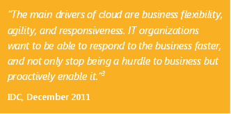
Undeniably, cloud computing represents a major shift happening in IT today. Yesterday, the conversation was about consolidation and cost. Today, it’s about the new class of benefits that cloud computing can deliver. It’s all about transforming the way IT serves organizations by harnessing a new breed of power. Cloud computing is fundamentally changing the world of IT, impacting every role—from service providers and system architects to developers and end users.

Research shows that agility, focus, and economics are three top drivers for cloud adoption:

  • Agility: Cloud computing can speed an organization’s ability to capitalize on new opportunities and respond to changes in business demands.
  • Focus: Cloud computing enables IT departments to cut infrastructure costs dramatically. Infrastructure is abstracted and resources are pooled, so IT runs more like a utility than a collection of complicated services and systems. Plus, IT now can be transitioned to more innovative and strategic roles.
  • Economics: Cloud computing reduces the cost of delivering IT and increases the utilization and efficiency of the data center. Delivery costs go down because with cloud computing, applications and resources become self-service, and use of those resources becomes measurable in new and precise ways. Hardware utilization also increases because infrastructure resources (storage, compute, and network) are now pooled and abstracted.

Delivery Models for Cloud Services

In simple terms, cloud computing is the abstraction of IT services. These services can range from basic infrastructure to complete applications. End users request and consume abstracted services without the need to manage (or even completely know about) what constitutes those services. Today, the industry recognizes three delivery models for cloud services, each providing a distinct trade-off between control/flexibility and total cost:

  • Infrastructure as a Service (IaaS): Virtual infrastructure that hosts virtual machines and mostly existing applications.
  • Platform as a Service (PaaS): Cloud application infrastructure that provides an on-demand application-hosting environment.
  • Software as a Service (SaaS): Cloud services model where an application is delivered over the Internet and customers pay on a per-use basis (for example, Microsoft Office 365 or Microsoft CRM Online).

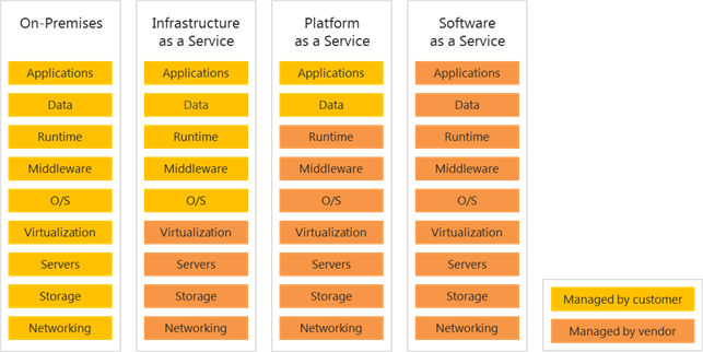
Figure 1 depicts the cloud services taxonomy and how it maps to the components in an IT infrastructure. With an on-premises model, the customer is responsible for managing the entire stack—ranging from network connectivity to applications. With IaaS, the lower levels of the stack are managed by a vendor, while the customer is responsible for managing the operating system through applications. With PaaS, a platform vendor provides and manages everything from network connectivity through runtime. The customer only needs to manage applications and data. (The Windows Azure offering best fits in this model.) Finally, with SaaS, a vendor provides the applications and abstracts all services from all underlying components.

Figure 1: Cloud services taxonomy


Windows Azure Virtual Machines

Windows Azure Virtual Machines introduce functionality that allows full control and management of VMs, along with extensive virtual networking. This offering can provide organizations with robust benefits, such as:

  • Management: Centrally manage VMs in the cloud with full control to configure and maintain the infrastructure.
  • Application mobility: Move virtual hard drives (VHDs) back and forth between on-premises and cloud-based environments. There is no need to rebuild applications to run in the cloud.
  • Access to Microsoft server applications: Run the same on-premises applications and infrastructure in the cloud, including Microsoft SQL Server, SharePoint Server, Windows Server, and Active Directory.

Windows Azure Virtual Machines is an easy, open and flexible, and powerful platform that allows organizations to deploy and run Windows Server and Linux VMs in minutes:

  • Easy: With Windows Azure Virtual Machines, it is easy and simple to build, migrate, deploy, and manage VMs in the cloud. Organizations can migrate workloads to Windows Azure without having to change existing code, or they can set up new VMs in Windows Azure in only a few clicks. The offering also provides assistance for new cloud application development by integrating the IaaS and PaaS functionalities of Windows Azure.
  • Open and flexible: Windows Azure is an open platform that gives organizations flexibility. They can start from a prebuilt image in the image library, or they can create and use customized and on-premises VHDs and upload them to the image library. Community and commercial versions of Linux also are available.
  • Powerful: Windows Azure is an enterprise-ready cloud platform for running applications such as SQL Server, SharePoint Server, or Active Directory in the cloud. Organizations can create hybrid on-premises and cloud solutions with VPN connectivity between the Windows Azure data center and their own networks.

SharePoint on Windows Azure Virtual Machines

SharePoint 2010 flexibly supports most of the workloads in a Windows Azure Virtual Machines deployment. Windows Azure Virtual Machines are an optimal fit for FIS (SharePoint Server for Internet Sites) and development scenarios. Likewise, core SharePoint workloads are also supported. If an organization wants to manage and control its own SharePoint 2010 implementation while capitalizing on options for virtualization in the cloud, Windows Azure Virtual Machines are ideal for deployment.

The Windows Azure Virtual Machines offering is hosted and managed in the cloud. It provides deployment flexibility and reduces cost by mitigating capital expenditures due to hardware procurement. With increased infrastructure agility, organizations can deploy SharePoint Server in hours—as opposed to days or weeks. Windows Azure Virtual Machines also enables organizations to deploy SharePoint workloads in the cloud using a “pay-as-you-go” model.
As SharePoint workloads grow, an organization can rapidly expand infrastructure; then, when computing needs decline, it can return the resources that are no longer needed—thereby paying only for what is used.

Shift in IT Focus

Many organizations contract out the common components of their IT infrastructure and management, such as hardware, operating systems, security, data storage, and backup—while maintaining control of mission-critical applications, such as SharePoint Server. By delegating all non-mission-critical service layers of their IT platforms to a virtual provider, organizations can shift their IT focus to core, mission-critical SharePoint services and deliver business value with SharePoint projects, instead of spending more time on setting up infrastructure.

Faster Deployment

Supporting and deploying a large SharePoint infrastructure can hamper IT’s ability to move rapidly to support business requirements. The time that is required to build, test, and prepare SharePoint servers and farms and deploy them into a production environment can take weeks or even months, depending on the processes and constraints of the organization. Windows Azure Virtual Machines allow organizations to quickly deploy their SharePoint workloads without capital expenditures for hardware. In this way, organizations can capitalize on infrastructure agility to deploy in hours instead of days or weeks.

Scalability

Without the need to deploy, test, and prepare physical SharePoint servers and farms, organizations can expand and contract compute capacity on demand, at a moment’s notice. As SharePoint workload requirements grow, an organization can rapidly expand its infrastructure in the cloud. Likewise, when computing needs decrease, the organization can diminish resources, paying only for what it uses. Windows Azure Virtual Machines reduces upfront expenses and long-term commitments, enabling organizations to build and manage SharePoint infrastructures at scale. Again, this means that these organizations can innovate, experiment, and iterate in hours—as opposed to days and weeks with traditional deployments.

Metered Usage

Windows Azure Virtual Machines provide computing power, memory, and storage for SharePoint scenarios, whose prices are typically based on resource consumption. Organizations pay only for what they use, and the service provides all capacity needed for running the SharePoint infrastructure. For more information on pricing and billing, go to Windows Azure Pricing Details. Note that there are nominal charges for storage and data moving out of the Windows Azure cloud from an on-premises network. However, Windows Azure does not charge for uploading data.

Flexibility

Windows Azure Virtual Machines provide developers with the flexibility to pick their desired language or runtime environment, with official support for .NET, Node.js, Java, and PHP. Developers also can choose their tools, with support for Microsoft Visual Studio, WebMatrix, Eclipse, and text editors. Further, Microsoft delivers a low-cost, low-risk path to the cloud and offers cost-effective, easy provisioning and deployment for cloud reporting needs—providing access to business intelligence (BI) across devices and locations. Finally, with the Windows Azure offering, users not only can move VHDs to the cloud, but also can copy a VHD back down and run it locally or through another cloud provider, as long as they have the appropriate license.

Provisioning Process

This subsection discusses the basic provisioning process in Windows Azure. The image library in Windows Azure provides the list of available preconfigured VMs. Users can publish SharePoint Server, SQL Server, Windows Server, and other ISO/VHDs to the image library. To simplify the creation of VMs, base images are created and published to the library. Authorized users can use these images to generate the desired VM. For more information, go to Create a Virtual Machine Running Windows Server 2008 R2 on the Windows Azure site. Figure 2 shows the basic steps for creating a VM using the Windows Azure Management Portal:

Figure 2: Overview of steps for creating a VM


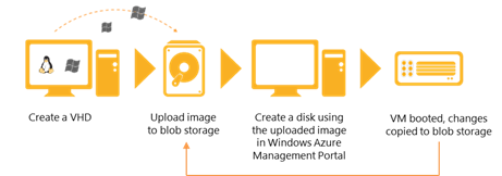
Users also can upload a sysprepped image on the Windows Azure Management Portal. For more information, go to Creating and Uploading a Virtual Hard Disk. Figure 3 shows the basic steps for uploading an image to create a VM:

Figure 3: Overview of steps for uploading an image

Deploying SharePoint 2010 on Windows Azure

You can deploy SharePoint 2010 on Windows Azure by following these steps:

  1. Log on to the Windows Azure (Preview) Management Portal through your account.
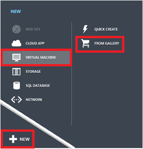
  1. Create a VM with base operating system: On the Windows Azure Management Portal, click +NEW, then click VIRTUAL MACHINE, and then click FROM GALLERY.

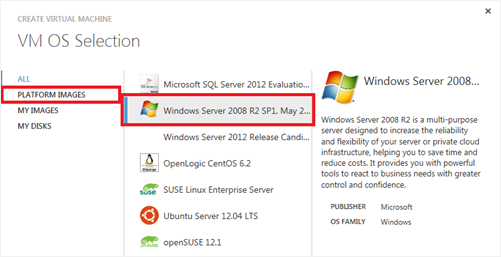
  2. The VM OS Selection dialog box appears. Click Platform Images, select the Windows Server 2008 R2 SP1 platform image.


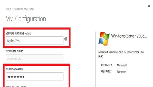
  1. The VM Configuration dialog box appears. Provide the following information:
  • Enter a VIRTUAL MACHINE NAME.
    • This machine name should be globally unique.
  • Leave the NEW USER NAME box as Administrator.
  • In the NEW PASSWORD box, type a strong password.
  • In the CONFIRM PASSWORD box, retype the password.
  • Select the appropriate SIZE.
    • For a production environment (SharePoint application server and database), it is recommended to use Large (4 Core, 7GB memory).

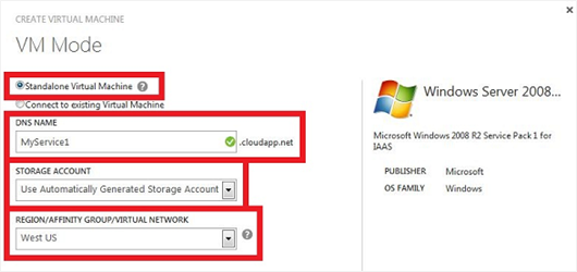
  1. The VM Mode dialog box appears. Provide the following information:
  • Select Standalone Virtual Machine.
  • In the DNS NAME box, provide the first portion of a DNS name of your choice.
    • This portion will complete a name in the format MyService1.cloudapp.net.
  • In the STORAGE ACCOUNT box, choose one of the following:
    • Select a storage account where the VHD file is stored.
    • Choose to have a storage account automatically created.
      • Only one storage account per region is automatically created. All other VMs created with this setting are located in this storage account.
      • You are limited to 20 storage accounts.
      • For more information, go to Create a Storage Account in Windows Azure.


  • In the REGION/AFFINITY GROUP/VIRTUAL NETWORK box, select the region where the virtual image will be hosted.

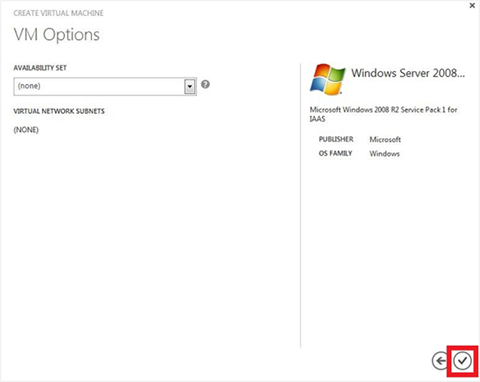
  1. The VM Options dialog box appears. Provide the following information:
  • In the AVAILABILITY SET box, select (none).
  • Read and accept the legal terms.
  • Click the checkmark to create the VM.


  1. The VM Instances page appears. Verify that your VM was created successfully.

  2. Complete VM setup:
  • Open the VM using Remote Desktop.
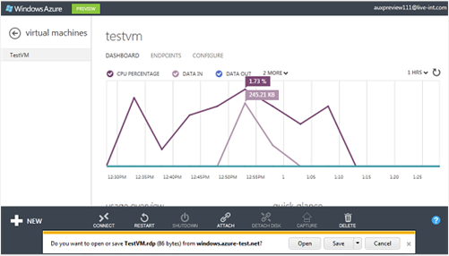
  • On the Windows Azure Management Portal, select your VM, and then select the DASHBOARD page.
  • Click Connect.

  1. Build the SQL Server VM using any of the following options:
  • Create a SQL Server 2012 VM by following steps 1 to 7 above—except in step 3, use the SQL Server 2012 image instead of the Windows Server 2008 R2 SP1 image. For more information, go to Provisioning a SQL Server Virtual Machine on Windows Azure.
    • When you choose this option, the provisioning process keeps a copy of SQL Server 2012 setup files in the C:\SQLServer_11.0_Full directory path so that you can customize the installation. For example, you can convert the evaluation installation of SQL Server 2012 to a licensed version by using your license key.
  • Use the SQL Server System Preparation (SysPrep) tool to install SQL Server on the VM with base operating system (as shown above in steps 1 to 7). For more information, go to Install SQL Server 2012 Using SysPrep.
  • Use the Command Prompt to install SQL Server. For more information, go to Install SQL Server 2012 from the Command Prompt.
  • Use supported SQL Server media and your license key to install SQL Server on the VM with base operating system (as shown above in steps 1 to 7).
  1. Build the SharePoint farm using the following substeps:
  • Substep 1: Configure the Windows Azure subscription using script files.
  • Substep 2: Provision SharePoint servers by creating another VM with base operating system (as shown above in steps 1 to 7). To build a SharePoint server on this VM, choose one of the following options:
  • Substep 3: Configure SharePoint. After each SharePoint VM is in the ready state, configure SharePoint Server on each server by using one of the following options:
    • Configure SharePoint from the GUI.
    • Configure SharePoint using Windows PowerShell. For more information, go to Install SharePoint Server 2010 by Using Windows PowerShell.
      • You also can use the CodePlex Project’s AutoSPInstaller, which consists of Windows PowerShell scripts, an XML input file, and a standard Microsoft Windows batch file. AutoSPInstaller provides a framework for a SharePoint 2010 installation script based on Windows PowerShell. For more information, go to CodePlex: AutoSPInstaller.

  1. After the script gets completed, connect to the VM using the VM Dashboard.
  2. Verify SharePoint configuration: Log on to the SharePoint server, and then use Central Administration to verify the configuration.

Creating and Uploading a Virtual Hard Disk

You also can create your own images and upload them to Windows Azure as a VHD file. To create and upload a VHD file on Windows Azure, follow these steps:

  1. Create the Hyper-V-enabled image: Use Hyper-V Manager to create the Hyper-V-enabled VHD. For more information, go to Create Virtual Hard Disks.
  2. Create a storage account in Windows Azure: A storage account in Windows Azure is required to upload a VHD file that can be used for creating a VM. This account can be created using the Windows Azure Management Portal. For more information, go to Create a Storage Account in Windows Azure.
  3. Prepare the image to be uploaded: Before the image can be uploaded to Windows Azure, it must be generalized using the SysPrep command. For more information, go to How to Use SysPrep: An Introduction.
  4. Upload the image to Windows Azure: To upload an image contained in a VHD file, you must create and install a management certificate. Obtain the thumbprint of the certificate and the subscription ID. Set the connection and upload the VHD file using the CSUpload command-line tool. For more information, go to Upload the Image to Windows Azure.


Usage Scenarios

This section discusses some leading customer scenarios for SharePoint deployments using Windows Azure Virtual Machines. Each scenario is divided into two parts—a brief description about the scenario followed by steps for getting started.

Scenario 1: Simple SharePoint Development and Test Environment

Description

Organizations are looking for more agile ways to create SharePoint applications and set up SharePoint environments for onshore/offshore development and testing. Fundamentally, they want to shorten the time required to set up SharePoint application development projects, and decrease cost by increasing the use of their test environments. For example, an organization might want to perform on-demand load testing on SharePoint Server and execute user acceptance testing (UAT) with more concurrent users in different geographic locations. Similarly, integrating onshore/offshore teams is an increasingly important business need for many of today’s organizations.

This scenario explains how organizations can use preconfigured SharePoint farms for development and test workloads. A SharePoint deployment topology looks and feels exactly as it would in an on-premises virtualized deployment. Existing IT skills translate 1:1 to a Windows Azure Virtual Machines deployment, with the major benefit being an almost complete cost shift from capital expenditures to operational expenditures—no upfront physical server purchase is required. Organizations can eliminate the capital cost for server hardware and achieve flexibility by greatly reducing the provisioning time required to create, set up, or extend a SharePoint farm for a testing and development environment. IT can dynamically add and remove capacity to support the changing needs of testing and development. Plus, IT can focus more on delivering business value with SharePoint projects and less on managing infrastructure.

To fully utilize load-testing machines, organizations can configure SharePoint virtualized development and test machines on Windows Azure with operating system support for Windows Sever 2008 R2. This enables development teams to create and test applications and easily migrate to on-premises or cloud production environments without code changes. The same frameworks and toolsets can be used on premises and in the cloud, allowing distributed team access to the same environment. Users also can access on-premises data and applications by establishing a direct VPN connection.

Getting Started

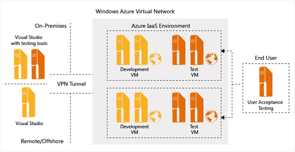
Figure 4 shows a SharePoint development and testing environment in a Windows Azure VM. To build this deployment, start by using the same on-premises SharePoint development and testing environment used to develop applications. Then, upload and deploy the applications to the Windows Azure VM for testing and development. If your organization decides to move the application back on-premises, it can do so without having to modify the application.


Figure 4: SharePoint development and testing environment in Windows Azure Virtual Machines


Setting Up the Scenario Environment

To implement a SharePoint development and testing environment on Windows Azure, follow these steps:

  1. Provision: First, provision a VPN connection between on-premises and Windows Azure using Windows Azure Virtual Network. (Because Active Directory is not being used here, a VPN tunnel is needed.) For more information, go to Windows Azure Virtual Network (Design Considerations and Secure Connection Scenarios). Then, use the Management Portal to provision a new VM using a stock image from the image library.
  • You can upload the on-premises SharePoint development and testing VMs to your Windows Azure storage account and reference those VMs through the image library for building the required environment.
  • You can use the SQL Server 2012 image instead of the Windows Server 2008 R2 SP1 image. For more information, go to Provisioning a SQL Server Virtual Machine on Windows Azure.
  1. Install: Install SharePoint Server, Visual Studio, and SQL Server on the VMs using a Remote Desktop connection.
  1. Develop deployment packages and scripts for applications and databases: If you plan to use an available VM from the image library, the desired on-premises applications and databases can be deployed on Windows Azure Virtual Machines:
  • Create deployment packages for the existing on-premises applications and databases using SQL Server Data Tools and Visual Studio.
  • Use these packages to deploy the applications and databases on Windows Azure Virtual Machines.
  1. Deploy SharePoint applications and databases:
  • Configure security on the Management Portal endpoint and set an inbound port in the VM’s Windows Firewall.
  • Deploy SharePoint applications and databases to Windows Azure Virtual Machines using the deployment packages and scripts created in step 3.
  • Test deployed applications and databases.
  1. Manage VMs:
  • Monitor the VMs using the Management Portal.
  • Monitor the applications using Visual Studio and SQL Server Management Studio.
  • You also can monitor and manage the VMs using on-premises management software, like Microsoft System Center – Operations Manager.

Scenario 2: Public-facing SharePoint Farm with Customization

Description

Organizations want to create an Internet presence that is hosted in the cloud and is easily scalable based on need and demand. They also want to create partner extranet websites for collaboration and implement an easy process for distributed authoring and approval of website content. Finally, to handle increasing loads, these organizations want to provide capacity on demand to their websites.

In this scenario, SharePoint Server is used as the basis for hosting a public-facing website. It enables organizations to rapidly deploy, customize, and host their business websites on a secure, scalable cloud infrastructure. With SharePoint public-facing websites on Windows Azure, organizations can scale as traffic grows and pay only for what they use. Common tools, similar to those used on premises, can be used for content authoring, workflow, and approval with SharePoint on Windows Azure.

Further, using Windows Azure Virtual Machines, organizations can easily configure staging and production environments running on VMs. SharePoint public-facing VMs created in Windows Azure can be backed up to virtual storage. In addition, for disaster recovery purposes, the Continuous Geo-Replication feature allows organizations to automatically back up VMs operating in one data center to another data center miles away. (For more information on geo-replication, go to Introducing Geo-replication for Windows Azure Storage).

VMs in Windows Azure infrastructure are validated and supported for working with other Microsoft products, such as SQL Server and SharePoint Server. Windows Azure and SharePoint Server are better together: Both are part of the Microsoft family and are thoroughly integrated, supported, and tested together to provide an optimal experience. They both have a single point of support for the SharePoint application and the Windows Azure infrastructure.

Getting Started

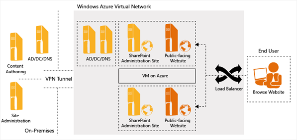
In this scenario, more front-end web servers for SharePoint Server must be added to support extra traffic. These servers require enhanced security and Active Directory Domain Services domain controllers to support user authentication and authorization. Figure 5 shows the layout for this scenario.

Figure 5: Public-facing SharePoint farm with customization


Setting Up the Scenario Environment

To implement a public-facing SharePoint farm on Windows Azure, follow these steps:

  1. Deploy Active Directory: The fundamental requirements for deploying Active Directory on Windows Azure Virtual Machines are similar—but not identical—to deploying it on VMs (and, to some extent, physical machines) on-premises. For more information about the differences, as well as guidelines and other considerations, go to Guidelines for Deploying Active Directory on Windows Azure Virtual Machines. To deploy Active Directory in Windows Azure:
  1. Provision a VM: Use the Management Portal to provision a new VM from a stock image in the image library.
  2. Deploy a SharePoint farm:
  • Use the newly provisioned VM to install SharePoint and generate a reusable image. For more information about installing SharePoint Server, go to Install and Configure SharePoint Server 2010 by Using Windows PowerShell or CodePlex: AutoSPInstaller.
  • Configure the SharePoint VM to create and connect to the SharePoint farm.
  • Use the Management Portal to configure the load balancing.
    • Configure the VM endpoints, select the option to load balance traffic on an existing endpoint, and then specify the name of the load-balanced VM.
    • Add another front-end web VM to the existing SharePoint farm for extra traffic.
  1. Manage VMs:

  • Monitor the VMs using the Management Portal.
  • Monitor the SharePoint farm using Central Administration.

Scenario 3: Scaled-out Farm for Additional BI Services

Description

Business intelligence is essential to gaining key insights and making rapid, sound decisions. As organizations transition from an on-premises approach, they do not want to make changes to the BI environment while deploying existing BI applications to the cloud. They want to host reports from SQL Server Analysis Services (SSAS) or SQL Server Reporting Services (SSRS) in a highly durable and available environment, while keeping full control of the BI application—all without spending much time and budget on maintenance.

This scenario describes how organizations can use Windows Azure Virtual Machines to host mission-critical BI applications. Organizations can deploy SharePoint farms in Windows Azure Virtual Machines and scale out the application server VM’s BI components, like SSRS or Excel Services. By scaling resource-intensive components in the cloud, they can better and more easily support specialized workloads. Note that SQL Server in Windows Azure Virtual Machines performs well, as it is easy to scale SQL Server instances, ranging from small to extra-large installations. This provides elasticity, enabling organizations to dynamically provision (expand) or deprovision (shrink) BI instances based on immediate workload requirements.

Migrating existing BI applications to Windows Azure provides better scaling. With the power of SSAS, SSRS, and SharePoint Server, organizations can create powerful BI and reporting applications and dashboards that scale up or down. These applications and dashboards also can be more securely integrated with on-premises data and applications. Windows Azure ensures data center compliance with support for ISO 27001. For more information, go to the Windows Azure Trust Center.

Getting Started

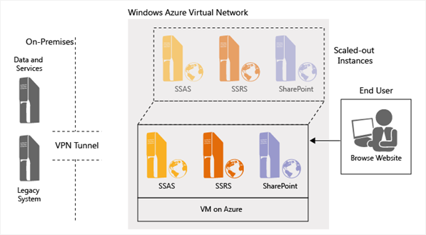
To scale out the deployment of BI components, a new application server with services such as PowerPivot, Power View, Excel Services, or PerformancePoint Services must be installed. Or, SQL Server BI instances like SSAS or SSRS must be added to the existing farm to support additional query processing. The server can be added as a new Windows Azure VM with SharePoint 2010 Server or SQL Server installed. Then, the BI components can be installed, deployed, and configured on that server (Figure 6).

Figure 6: Scaled-out SharePoint farm for additional BI services

Setting Up the Scenario Environment

To scale out a BI environment on Windows Azure, follow these steps:

  1. Provision:
  • Provision a VPN connection between on premises and Windows Azure using Windows Azure Virtual Network. For more information, go to Windows Azure Virtual Network (Design Considerations and Secure Connection Scenarios).
  • Use the Management Portal to provision a new VM from a stock image in the image library.
    • You can upload SharePoint Server or SQL Server BI workload images to the image library, and any authorized user can pick those BI component VMs to build the scaled-out environment.
  1. Install: If your organization does not have prebuilt images of SharePoint Server or SQL Server BI components, install SharePoint Server and SQL Server on the VMs using a Remote Desktop connection.
  1. Add the BI VM:
  • Configure security on the Management Portal endpoint and set an inbound port in the VM’s Windows Firewall.
  • Add the newly created BI VM to the existing SharePoint or SQL Server farm.
  1. Manage VMs:
  • Monitor the VMs using the Management Portal.
  • Monitor the SharePoint farm using Central Administration.
  • Monitor and manage the VMs using on-premises management software like Microsoft System Center – Operations Manager.

Scenario 4: Completely Customized SharePoint-based Website

Description

Increasingly, organizations want to create fully customized SharePoint websites in the cloud. They need a highly durable and available environment that offers full control to maintain complex applications running in the cloud, but they do not want to spend a large amount of time and budget.

In this scenario, an organization can deploy its entire SharePoint farm in the cloud and dynamically scale all components to get additional capacity, or it can extend its on-premises deployment to the cloud to increase capacity and improve performance, when needed. The scenario focuses on organizations that want the full “SharePoint experience” for application development and enterprise content management. The more complex sites also can include enhanced reporting, Power View, PerformancePoint, PowerPivot, in-depth charts, and most other SharePoint site capabilities for end-to-end, full functionality.

Organizations can use Windows Azure Virtual Machines to host customized applications and associated components on a cost-effective and highly secure cloud infrastructure. They also can use on-premises Microsoft System Center as a common management tool for on-premises and cloud applications.

Getting Started

To implement a completely customized SharePoint website on Windows Azure, an organization must deploy an Active Directory domain in the cloud and provision new VMs into this domain. Then, a VM running SQL Server 2012 must be created and configured as part of a SharePoint farm. Finally, the SharePoint farm must be created, load balanced, and connected to Active Directory and SQL Server (Figure 7).

Figure 7: Completely customized SharePoint-based website


Setting Up the Scenario Environment

The following steps show how to create a customized SharePoint farm environment from prebuilt images available in the image library. Note, however, that you also can upload SharePoint farm VMs to the image library, and authorized users can choose those VMs to build the required SharePoint farm on Windows Azure.

  1. Deploy Active Directory: The fundamental requirements for deploying Active Directory on Windows Azure Virtual Machines are similar—but not identical—to deploying it on VMs (and, to some extent, physical machines) on premises. For more information about the differences, as well as guidelines and other considerations, go to Guidelines for Deploying Active Directory on Windows Azure Virtual Machines. To deploy Active Directory in Windows Azure:
  1. Deploy SQL Server:
  • Use the Management Portal to provision a new VM from a stock image in the image library.
  • Configure SQL Server on the VM. For more information, go to Install SQL Server Using SysPrep.
  • Join the VM to the newly created Active Directory domain.
  1. Deploy a multiserver SharePoint farm:
  1. Manage the SharePoint farm through System Center:
  • Use the Operations Manager agent and new Windows Azure Integration Pack to connect your on-premises System Center to Windows Azure Virtual Machines.
  • Use on-premises App Controller and Orchestrator for management functions.


Conclusion

Cloud computing is transforming the way IT serves organizations. This is because cloud computing can harness a new class of benefits, including dramatically decreased cost coupled with increased IT focus, agility, and flexibility. Windows Azure is leading the way in cloud computing by delivering easy, open, flexible, and powerful virtual infrastructure. Windows Azure Virtual Machines mitigate the need for hardware, so organizations can reduce cost and complexity by building infrastructure at scale—with full control and streamlined management.

Windows Azure Virtual Machines provide a full continuum of SharePoint deployments. It is fully supported and tested to provide an optimal experience with other Microsoft applications. As such, organizations can easily set up and deploy SharePoint Server within Windows Azure, either to provision infrastructure for a new SharePoint deployment or to expand an existing one. As business workloads grow, organizations can rapidly expand their SharePoint infrastructure. Likewise, if workload needs decline, organizations can contract resources on demand, paying only for what they use. Windows Azure Virtual Machines deliver an exceptional infrastructure for a wide range of business requirements, as shown in the four SharePoint-based scenarios discussed in this paper.

Successful deployment of SharePoint Server on Windows Azure Virtual Machines requires solid planning, especially considering the range of critical farm architecture and deployment options. The insights and best practices outlined in this paper can help to guide decisions for implementing an informed SharePoint deployment.

Additional Resources

Guide to the Data Development Platform for . NET Developers

MSDN Library

.NET Development

Articles and Overviews

Data Access and Storage

ADO.NET

XML for Analysis Specification

Microsoft Data Development Technologies At a Glance

Guide to the Data Development Platform for .NET Developers

Hello, Data

Microsoft Data Development Technologies: Past, Present, and Future

OData by Example

Testability and Entity Framework 4.0


Guide to the Data Development Platform for .
NET Developers


SQL Server Technical Article

Published: November 2009

Applies to: SQL Server 2008

Summary: This whitepaper covers all facets of the .NET data development platform. This includes both client-side and service-based APIs but also .NET APIs for programming at a server level inside the SQL Server 2008 database and for developing and testing a SQL Server database application. It also includes information on future directions of the .NET and SQL Server development platform.

Introduction

The large majority of applications use a database to store, query, and maintain their data. Almost all of them use a relational database that is designed using the principals of data normalization and queried with set-based queries using the SQL query language.  Application programmers need to tie user activities, such as ordering products and browsing through lists of items for sale, to database activities like SELECT statements and stored procedure execution in a visually pleasing and responsive graphical user interface. They need data access and data binding to the user interface that is encapsulated in easy-to-use components that employ the same object-oriented concepts that are used in the rest of the application. To develop responsive, robust applications on-time and on-budget, programmers need to reduce the time from model to implementation, as well as to easily write automated test cases to ensure the application is robust and scalable.

But data usage doesn’t end there.  One of the key challenges today is to make sense of the data in timely manner.  This means applications often add Business Intelligence to the OLTP (online transaction processing system) data that is managed in a relational database for timely decision making within OLTP applications. The OLTP data can be imported, exported, combined with other data and transformed using ETL (extract, transform, and load) technologies, and analyzed using an OLAP (online analytical processing) system. Patterns and insights can be teased from the data using smart data mining algorithms. User interactions can be real-time, but reports serve an important role in data presentation and can be embellished graphically using charts, gauges, maps and other user-interface controls.  Programmers enhancing applications with Business Intelligence should be able to leverage existing experience by using the same basic programming APIs and methodology as they use in application development.

Since the .NET framework 1.0 was released in 2002, it has become programmers’ preferred framework for developing software, including data-driven applications, on Microsoft platforms. .NET 1.0 includes a set of classes known as ADO.NET to provide a substrate for database development. ADO.NET is based on a provider model. Databases products (like SQL Server, Oracle, and DB2) hook into the model by delivering their own data provider. .NET 1.0 shipped with three data providers; bridge providers to existing ODBC drivers and OLE DB providers, and the SqlClient provider for the SQL Server database. Over time, not only has the SqlClient provider been improved to keep pace with innovations in the SQL Server database, but SQL Server has expanded the number of integration points between the database and its related features and the .NET framework. Today .NET APIs are an integral part of the SQL Server product. In this whitepaper, I’ll describe the current state of the Microsoft Data Development Platform and illustrate the deep integration between .NET and SQL Server to show why SQL Server is the preferred database product for .NET developers. The .NET database platform has been enhanced since the advent of .NET to include functionality like object-relational mapping and a programming language integrated query language.  I’ll also discuss the direction that platforms and integration will take in the future so you can plan your overall database development strategy.

Flexible Data Access Frameworks for Productive .NET Application Development

Data Access Frameworks are what developers normally consider to be “database programming”.  .NET developers have a choice of using the low-level ADO.NET object model or the higher-level conceptual model as defined by the ADO.NET Entity Framework. You can also program you client-level database access using through a well-known REST-based services model, exposing the database as a service in the world of Software As A Service. Each of the client-level data access frameworks integrate seamlessly with multi-tier applications and with visual controls in the .NET platform.

ADO.NET – The Substrate

ADO.NET is the base database API and the basis for all of today’s .NET-based data access frameworks. All existing .NET applications in releases prior to .NET 3.5 use this API. Programmers should use ADO.NET when they want direct control of the SQL statements used to communicate with the underlying database and also to access specific database features not supported by the ADO.NET Entity Framework.

Microsoft ships three SQL Server-related ADO.NET data providers. System.Data.SqlClient is the provider for the SQL Server database engine, mentioned previously. Microsoft.Data.SqlCe is a provider for SQL Server Compact Edition that works on the desktop or on compact devices. There is also a specialized data provider for SQL Server Analysis Services and Data Mining functionality (the ADOMD.NET provider), which will be mentioned later.

 ADO.NET uses the “connection-command-resultset” paradigm. Programmers open a Connection to the database, and issue Commands consisting of stored procedures or SQL statements that can either perform insert, update, and delete operations, or select statements that return a DataReader (resultset). Additional classes encapsulate transactions, procedure parameters, and error handling. ADO.NET 1.0 and 1.1 used an interface-based design; that is, programmers used database-specific classes that implemented the well-known IDbConnection, IDbCommand, and IDataReader interfaces. ADO.NET 2.0 added base classes so database-specific classes derived from the generic DbConnection, DbCommand, and DbDataReader classes. The base classes or interfaces provide the generic functionality; database-specific functionality is encapsulated in provider-specific classes (e.g. SqlConnection, SqlCommand, and SqlDataReader). For more information reference “Generic Coding with ADO.NET 2.0 Base Classes and Factories” at http://msdn.microsoft.com/en-us/library/ms379620(VS.80).aspx.

Database transactions are accommodated in the model in two ways. Local transactions can be represented by a DbTransaction object which is specified as a property of the connection object. Alternatively, .NET developers can use the System.Transactions library. System.Transactions supports local and distributed transactions and passes and tracks transactions through an instance of the TransactionScope class.

The specific server, database, and other connection parameters are specified in a connection string. The preferred method for specifying a connection string is to include it in the application’s .NET configuration (.config) file. There is a standard configuration file location used for ADO.NET connection strings.

Programmers use the .NET type system in their applications, but relational data types in the database, so there needs to be a low-level .NET type system-to-database type system correspondence. Database types mostly follow the ISO-ANSI SQL standard type system, but database vendors can include database-specific types. In ADO.NET, common database types are represented using an enumeration for the common types, System.Data.DbTypes. Programmers rely on documented mapping of their database’s data type to DbTypes, but providers can also add database-specific types.  SqlClient accommodates SQL Server-specific types by using a SqlDbTypes enumeration. A type correspondence mismatch occurs because most types in the .NET type system have nothing that distinguishes database NULL from empty instance of a type. A set of SQL Server-specific types in the System.Data.SqlTypes namespace not only encapsulate the concept of database NULL by implementing an INullable interface, but are isomorphic with the data types in SQL Server. .NET 2.0 adds a generic nullable type that works with .NET value types (structures). Nullable types can be used as an alternative to System.Data.SqlTypes.

The SqlClient provider is the lowest-level .NET data access APIs and also the closest to SQL Server. It is the only client database API that supports all of the latest enhancements in SQL Server. Programmers must use native ADO.NET calls when they need access to these features. For example, only ADO.NET and SqlClient directly support the Filestream storage with streaming I/O and the table-valued parameters features of SQL Server 2008. SqlClient is also the only database API to directly support SQL Server data types implemented in .NET, such as SQL Server 2008’s spatial data types and hierarchyid type, as well as SQL Server UDTs (user-defined types) implemented in .NET in the server and on the client. The SQL Server and .NET teams work closely together; an example of this is the introduction a new .NET primitive type, the System.DateTimeOffset data type in .NET 3.5 that corresponds to SQL Server 2008’s datetimeoffset data type. This makes it straightforward for programmers to take advantage of the very latest SQL Server features.

ADO.NET also provides for a “disconnected update” scenario using a class called the DataSet that contains of collection of DataTable instances with collections of DataRow and DataColumn objects. The DataSet interacts with the database through a DataAdapter class, and includes relational database-like features such as indexing, primary keys, defaults, identity columns, and constraints, including referential constraints between DataTables. Programmers can use the DataSet as an in-memory object model for database data, although with the advent of the ADO.NET Entity Framework a model based on entities is preferred because you program against business objects rather than a relational-style object model.

LINQ – Native Data Querying integrated into .Net Languages

LINQ is a SQL-like, strongly-typed, query language that is implemented using built-in programming language constructs in .NET. This provides the ability to query any implementation of a .NET IEnumerable<T> class using SQL syntax. LINQ defines a standard set of query operators that allow both set-based (e.g. projection, selection) and cursor-based (e.g. traversal) queries using programming language syntax. LINQ uses a provider model to allow access to domain-specific stores such as relational database, XML, Windows Active Directory, collections of objects, and ADO.NET DataSets. In most cases, the providers work by translating LINQ queries to queries against the domain-specific store.

These Using LINQ queries that produce SQL query statements gives programmers compile-time syntax checking and IntelliSence, reduces data access coding time compared to coding with raw SQL strings, and also provides protection from SQL injection. This is an improvement for programmers who don’t use stored procedures and code SQL strings directly in application code, because these SQL strings are not syntax-checked by the underlying programming language compiler.

Two implementations of LINQ over ADO.NET were introduced in .NET 3.5. LINQ to SQL is a SQL Server-specific implementation over a collection of tables represented as objects. It includes a mapping tool that maps tables to objects, stored procedure support, and implements almost all LINQ operators by translating them into T-SQL. Programmers can insert, update, and delete rows from database tables through objects using a DataContext class, which extends the basic LINQ functionality.  A similar LINQ provider also exists for the SQL Server Compact Edition. 

Programmers use the ADO.NET DataSet object because it represents its data as a familiar collection of tables that contain columns and rows.  There is also a LINQ provider over the DataSet class that provides functionality not included in the original DataSet classes using standard SQL syntax. This implementation allows selection, projection, joins, and other LINQ operators against the DataSet’s collection of DataTables. Programmers that use the DataSet in existing applications can use the LINQ provider to extend the base functionality. Using LINQ to DataSet enhancements does not change the paradigm that filling the DataSet with database data and updating the database when changes are made to the DataSet is controlled by the DataAdapter class.

ADO.Net Entity Framework and the Entity Data Model Overcome the Object Relational Impedance Mismatch

Object-oriented programming concepts have taken hold in the development community, enjoying the same widespread popularity as the relational normalization-based design and set-based programming has in the database community. Therefore, there is a need to bridge the gap between relational sets to collections of objects and map operations on object instances to changes in the database. Programmers can bridge this gap, known as the object-relational impedance mismatch, by using the ADO.NET Entity Framework.

The ADO.NET Entity Framework should be considered the development API of choice for .NET SQL Server programmers going forward. The Entity Framework raises the abstraction level of data access from logical relational database-based access to conceptual model-based access. For more information on this, reference the whitepaper “Next-Generation Data Access: Making the Conceptual Level Real” at http://msdn.microsoft.com/en-us/library/aa730866(VS.80).aspx.

The Entity Framework consists of five main parts. These are the Entity Data Model (EDM), the EntityClient provider and Entity SQL language, the ObjectServices libraries, and the LINQ to Entities provider.

The Entity Data Model (EDM) specifies the conceptual model that you program against and it’s mapping to underlying database primitives. With EDM, programmers specify the classes and relationships that will be used in the object model (conceptual schema), how tuples and relations are represented in the database (physical schema), and how to map between the two (mapping schema). EDM directly supports table-per-type mapping as well as modeling inheritance using either table-per-hierarchy or table-per-concrete-type. But mapping supports more than just database tables. Mapping entities to stored procedure resultsets and projections as a ComplexType, database views, and on-the-fly projection mapping as anonymous types are also supported. The EDM is specified by using a Visual Studio designer against a set of XML schemas. This metadata can be represented as an XML file (edmx) which can compiled into a program resource.

Entity Framework is layered over ADO.NET and most ADO.NET data providers have been enhanced to work with it. Programmers can work directly with an Entity Data Model using ADO.NET by using the EntityClient provider. To use EntityClient, you specify both the Entity Data Model and the underlying data provider (e.g. SqlClient) in the ADO.NET connection string.

The entity framework defines a language called Entity SQL that extends traditional SQL with some additional object-oriented query constructs.  Entity SQL is the low-level query language of the Entity Framework that is used to query against the conceptual model.  Finally, the Entity Framework includes an implementation of the LINQ query language, known as LINQ to Entities. LINQ to Entities implements almost all of the constructs in Entity SQL.

You can program the Entity Framework using three different programming models: LINQ to Entities, ObjectServices, or “native” ADO.NET using the EntityClient provider. Both EntityClient and ObjectServices use Entity SQL strings directly. Although some lower-level query functionality can only be expressed using EntitySQL, using LINQ to Entities is the overwhelming favorite among programmers that use the Entity Framework. LINQ to Entities is preferred for most development because using LINQ query language instead of EntitySQL gives programmers compile-time syntax checking and IntelliSence, reducing coding time.

The Entity Framework includes a type system that supports Entity Types, Simple Types, Complex Types, and Row Types. Entity Types contain a reference to an instance of the type called an EntityKey. The set of supported Simple Types is a subset of data types found in most relational databases. A complex type is a set of multiple simple types, e.g. a resultset from a stored procedures or a projection from a SQL query. Entities and Associations between entities live in containers known as EntitySets and AssociationSets.  EntityContainer is the top level object that usually maps to a database or application’s scope.

The programming model supports insert, update, and delete operations against the entities by tracking changes with an ObjectContext. The model can generate the SQL required for these operations or they can be mapped to a set of user-written stored procedures. Both lazy and eager loading of related entities is supported. Transactions are accommodated by using System.Transactions.

Entity Framework 4.0, which will ship with .NET 4.0, adds a variety of new features that support a model-first methodology, test-driven development (make it easier to create a mocking layer for testing ), and persistence ignorance. In addition, there are improvements in the SQL generation layer, both in the translation of LINQ to Entities queries and in the SQL Server provider specifically that make the generated SQL more performant. EF 4.0 also directly supports a representation of foreign keys between entities which is useful for data binding.

ADO.NET Data Services – RESTful Data Access

All of the database client APIs that I’ve mentioned so far require a direct connection to the database from either the client or middle-tier. But popular programming models such as Silverlight and AJAX (Asynchronous Javascript and XML) interact with all data sources directly from browser code, using either XML or JSON (JavaScript Object Notation) payloads.  This pattern requires programmers to use a middle-tier service that’s exposed through either SOAP or REST-based APIs. ADO.NET Data Services is the database API that exposes the data as a REST-based Web Service. The service is a WCF-based (Windows Communication Foundation) service that exposes database operations through the standard HTTP operations against a REST endpoint like GET, POST, PUT, and DELETE.

ADO.NET Data Services can use an Entity Framework model as an endpoint directly. It’s also able to work with other LINQ-based data sources (including LINQ to SQL) for reading. If you would like your non- EF data source to be available over ADO.NET data services for updating, you must provide an implementation of the IUpdateable interface.  SQL clauses like the WHERE, GROUP BY, and ORDER BY clause are implemented as parameters on the URL.

ADO.NET Data Services exposes entities (or any sets of data, such as SharePoint lists in SharePoint 2010) as either ATOMPub feeds (ATOM is a standard XML format used for data feeds) or collections of JSON objects. JSON objects are especially useful with AJAX clients. Because security needs to be considered in any service available on the Internet, granular data access security is enabled by using a set of data access expressions coded in the InitializeService method in combination with the authentication and authorization scheme of your choice. By default, no resources or associations are available unless you override the default InitializeService implementation. To build a robust application, ADO.NET Data Services clients may also require metadata; that is, information about the data available through a specific service endpoint.  A REST resource endpoint that supplies metadata for discovery purposes is also part of the model.

In addition to the capability to serve data, ADO.NET Data Services includes a client consumer API. In this API, the client “connects” to the endpoint by using the REST URL. Programmers query the data with a special LINQ provider that fetches updateable EDM object instances. This pattern encapsulates ADO.NET Data Services access so that it looks more like traditional data access code rather than raw HTTP and XML calls.

Programmers can use rich application frameworks that start with ADO.NET Data Services as a REST-based substrate for interacting with a database. One such framework is ASP.NET Dynamic Data, a template-based framework that allows you to build a data driven application quickly. It can use ADO.NET Data Services and LINQ to SQL or Entity Framework to access the relational database. Another framework is .NET RIA Services, which provides a set of components that allow building rich Internet applications (hence the acronym) using common patterns in ASP.NET, service-oriented architecture, and Silverlight 3.0 as a graphic user interface. It includes a pair of service models that hook directly into the ADO.NET Entity Framework, LINQ to SQL, or ADO.NET Data Services. This allows for data to be fetched though a service (a la ASP.NET AJAX) and bound to Silverlight data controls. These are mapped by .NET RIA Services to database maintenance functionality in the service models. .NET RIA Services is currently part of Visual Studio 2010 Beta2.

Harness your .Net skills within the Database for Scalable, Reliable and Manageable Applications

Data access APIs are normally considered as programming outside the database server. A specific database product, such as SQL Server, exposes programming models for in-server programming as well. Beginning with SQL Server 2005, SQL Server permitted in-server programming of database objects such as user-defined functions using .NET APIs as addition to traditional programming in native database languages such as SQL, MDX , and DMX. In addition, SQL Server provides mechanisms to extend and customize the product itself using .NET APIs, and .NET support extends deep into all facets of the server product. With SQL Server as the database, programmers can leverage their existing knowledge of .NET programming to add value to existing applications and also leverage knowledge of .NET APIs such as ADO.NET, which can be used both “outside” and “inside” the server. .NET integration with the database engine includes support for both application programmers and database administrators.

Programming SQL Server with .NET

Since SQL Server 2005, programmers have had the ability to incorporate .NET in database object code as an adjunct and alternative to using T-SQL. Hosting .NET code inside the SQL Server engine (that is, using SQL Server as a .NET runtime host) is commonly referred to as “SQLCLR”. One use of this .NET support is as a means to access external resources such as the registry or file system directly from database code, without resorting to unsafe mechanisms such as enabling xp_cmdshell or using undocumented system extended stored procedures. In addition, the programmer has a choice of .NET or T-SQL when writing user-defined functions, stored procedures and triggers. This allows a choice of best-of-breed mechanisms, that is, the ability to use .NET code where it’s more performant (such as regular expressions and complex calculations) and T-SQL when it’s more performant (database access and complex joins).

The SQL server team designed its .NET integration with security and reliability in mind, as well as performance. Safe SQLCLR code is limited to a subset of system assemblies that have been hardened and tested with SQL Server. These assemblies are guaranteed not to leak memory or other external resources, such as file handles, by the use of such coding primitives as SafeHandle and ConstrainedExecutionRegion introduced in .NET 2.0. Changes to the .NET 2.0 hosting APIs allow .NET resources such as memory allocation, thread pooling and scheduling, and exception handling, to be controlled by and integrated with the rest of the SQL Server engine. SQLCLR code runs in process, as part of the SQL Server service process (sqlservr.exe) for best performance, not in a separate service process.

Data access in SQLCLR database objects follows the ADO.NET object model with optimizations for in-server processing. SQLCLR code can directly execute T-SQL code, rather than requiring a separate ODBC or OLE DB connection (as extended stored procedures require) that use more memory and must be enlisted in the current transaction manually. This is accomplished by using a mechanism to give the appearance of an ordinary SqlConnection instance, but hook up memory pointers for direct access to database buffers, parameters, transaction space, and lock space. The SQLCLR code is part of the current connection. This internal connection is requested by a special connection string parameter “Context Connection=true”.

Server-side programmers use the SqlClient provider and the traditional Connection-Command-DataReader paradigm with a few extensions to accommodate server-specific constructs. This not only lets programmers familiar with ADO.NET leverage their existing expertise, but also allows the production of data access code that’s relatively portable from in-server to middle-tier and even to client should the need arise, with few changes to the code. The additional constructs for server-side code include a SqlContext and DbDataRecord. The SqlContext provides access to the code executor’s identity for access to external resources and a reference to a SqlPipe object. The SqlPipe is used to directly output resultsets or messages.  The DbDataRecord allows the programmer to synthesize resultsets from external resources. You can use this to represent Web Service results or files as a resultset from a stored procedure. In ADO.NET 3.5 and SQL Server 2008 a collection of DbDataRecord objects can also be used to construct table-valued parameters in client code.  Server-side programmers can also write .NET-based table-valued user-defined functions that expose any computed or refactored data as a set, in keeping with the T-SQL set-based paradigm.

There is a well-defined mapping between SQL data types and .NET data types and SQLCLR code must adhere to the mapping to be interoperable with T-SQL code. Although this mapping is mostly the same as client-side data type mapping, some data types (e.g. varchar, the non-Unicode string data type) do not have direct .NET equivalents and these cannot be used in SQLCLR result sets or parameters. In addition, .NET data types that do not have SQL Server equivalents (e.g. System.Collections.Hashtable) cannot be returned to T-SQL code, unless they are transformed into types (such as a collection of DbDataRecord objects returned from a stored procedure as a resultset) that T-SQL can work with.

Server-side programmers can also write SQLCLR user-defined aggregates and user-defined types (UDTs). User-defined aggregates extend the reach of aggregate functions to allow functions that are not built into T-SQL, such as covariant of a population. Programmers can use UDTs to create new scalar data types that extend the SQL Server type system.  UDTs and user-defined aggregates must be coded in SQLCLR, not T-SQL. The execution engine recognizes the new aggregate functions and includes them in the query plan, even allowing the aggregation function to be parallelized as with other query plan iterators.

Extended .Net Data Types and Code in SQL Server

In SQL Server 2008 some new features of the SQL Server engine itself were written in .NET code.  The new Policy Based Management and Change Data Capture features use .NET internally. This indicates that the SQL Server team has made a commitment to use SQLCLR code as an adjunct to unmanaged code where it is useful. Although there is a database option to disallow user-written SQLCLR code, this does not prevent the execution of system CLR code which is always enabled. Thus, in SQL Server 2008, .NET code is used as part of the engine’s standard operating environment.

Three new data types were introduced in SQL Server 2008 that are implemented using the SQLCLR user-defined type architecture; these are the spatial data types, geometry and geography, and the hierarchyid data type. The code that implements these data types in contained in a .NET assembly, Microsoft.SqlTypes.Types.dll. This assembly is required for normal server operation.  One reason for the implementation is that many different operations can be performed on these data types, especially the spatial types and the natural way to expose these is through type-specific methods.  The geometry data type, for example, has over 60 domain-specific methods and many properties that can be manipulated with the SQL-1999 standard “instance.method” syntax in T-SQL, instead of including a library of system functions that apply only to a single data type. This serves to better encapsulate the data type’s functionality.

Implementing built-in data types in .NET code also provides benefits for programmers that use the types. Firstly, the programming model for these types is identical whether you’re writing a SQL query or client-side object manipulation code.  This allows server programmers writing SQL with the instance.method syntax to leverage their expertise when writing either client code or SQLCLR stored procedures. In addition, Microsoft.SqlTypes.Types is distributable as part of the SQL Server Feature Pack, and useable directly on the client-side (in map-drawing applications for example) without a need to connect to the server at all. The server is used for data storage, SQL queries that may include spatial functions, and spatial indexing.

Programmatic Management with SQL Server Management Objects

.NET is used in programming administrative functions in the SQL Server Engine as well through the SQL Server Management Objects (SMO) libraries. SMO is a set of libraries that are used to manipulate and manage database objects (e.g. create a new database, configure network protocols, backup and restore the database). These libraries are used by SQL Server Management Studio (SSMS) Object Explorer and are available to programmers and administrators as well. This provides an additional choice to manage the database, serving as an alternative to SQL DDL statements and system stored procedures. Because they are used to write the SQL Server Management Studio utility, internal Policy Based Management code, and SQL Server Configuration Manager, the SMO libraries are quite comprehensive. These libraries also contain a special Scripter class that can be used to produce a SQL DDL script for any supported database object. This functionality is used extensively in SSMS. The two main functions of the library are DDL type operations and configuration operations in which the library is actually a .NET wrapper around WMI (Windows Management Instrumentation) operations. In addition, there is a set of classes that enable creating and controlling trace objects and a set of classes for creating and managing SQL Server Agent jobs. SQL Server also ships with a .NET library for configuring replication. The RMO (Replicate Management Objects) library can be used as an alternative to the system stored procedures for configuring SQL Server replication.

PowerShell Support in SQL Server

SQL Server 2008 introduced support for PowerShell, a new Windows shell and successor to the command shell. This product is part of the Microsoft Common Engineering Criteria and is supported as an administrative interface by almost every product in the Windows platform. IIS, Exchange, and Active Directory are parts of the platform that currently ship with PowerShell support. Third-party products such as VMWare are beginning to provide PowerShell support as well.

Because systems administrators or programmers often assume database administrator responsibilities in smaller installations and PowerShell is a common administration tool it is thought that “multi-product administrators” will leverage their PowerShell expertise to manage SQL Server, while specialized SQL Server-only DBAs will continue to use SQL scripts and system stored procedures. Experience with .NET object models is a useful skill when working in the PowerShell environment.

PowerShell is based on programming and scripting objects, rather than passing text between commands in scripts as traditional shells (e.g. CMD, csh) do. PowerShell uses cmdlets to manipulate the system; these are programmed in .NET code. In addition, products can expose administrative functionality through a provider model. PowerShell providers assist in generic knowledge transfer by representing system configuration using the file system paradigm combined with a standard set of operations such create-alter-delete on product nodes. SQL Server 2008 includes both cmdlets and a provider. SQL Server ships a custom shell (named SQLPS.exe) in which the cmdlets and the provider are pre-installed to prevent naming conflicts. You can also manually install the cmdlets and provider for use in the main PowerShell shell.

The provider exposes a few directories under the SQLSERVER: virtual directory.

  • SQL  – The SQL database engine objects (servers, databases, tables)
  • SQLPolicy – SQL Server policy-based management
  • SQLRegistration – Server registrations in SSMS
  • DataCollection –  Data collection for the Management Data Warehouse

   In SQL Server 2008 R2, two additional subdirectories are added

  • SQLUtility –The SQL Server Utility (Enterprise Multi-Server Management)
  • SQLDAC –DAC (Data-tier application databases)

There are only a few cmdlets in SQL Server 2008, including cmdlets for mapping between SQL Server database object names and PowerShell object names, a cmdlet with similar functionality to SQLCMD and cmdlets for executing policy-based management functions. Because the provider uses SMO objects to represent database objects internally, programming in PowerShell with SQL Server consists of quite a bit of navigation to the appropriate place in the provider virtual directory and then using SMO objects to perform operations.

The ability to use the SSMS Object Explorer context menu to bring up a PowerShell window at the appropriate position in the database object provider hierarchy as well as the ability to invoke PowerShell script as a SQL Agent job step round out the SQL Server 2008 PowerShell support.

Enrich your Applications with Embedded Business Intelligence

Business Intelligence is a set of tools and technologies designed to improve business decision making and planning. It generally includes reporting, quantitative analysis, and predictive modeling. Programmers can use their .NET skills along with tools in SQL Server in the programming of decision support systems.

.NET APIs are not only integrated with the database engine, but are pervasive in every part of the SQL Server product. .NET is used for four main Business Intelligence functionality groups:

  • Programming Business Intelligence client applications
  • Application programming at the server product level
  • Administration and Configuration programming
  • Writing product extensions

In this section, I’ll briefly describe the .NET facilities used by SQL Server Reporting Services (SSRS), SQL Server Analysis Services (SSAS), and SQL Server Integration Services (SSIS).

Integrate Reports & Data Visualization within your application with SQL Server Reporting Services

SQL Server Reporting Services is the tool of choice for programming reports to display in custom Web or Windows applications using the ReportViewer control , or publication in a central repository for convenient, secure, user access. Programmers can use SQL Server or Microsoft Office SharePoint Server as a repository or include report definitions directory in applications.  All of the entry points into the SSRS product allow programmers to leverage their .NET coding experience.

The report definition language (RDL) is a XML document format based on a published XML schema. SSRS reports are usually designed and published using Business Intelligence Development Studio (BIDS) or the graphic Report Builder tool. Reports can use Data Sources as input (SQL Server and a variety of other data sources are supported) and work with tables, views, and stored procedure data directly, or Report Models that expose metadata and relationships in a more user-friendly form. Report Models are designed and programmed in Visual Studio and can be generated against a SQL Server or Oracle database or an Analysis Services database.

The Report Manager is an ASP.NET-based application that allows administrators to manage reports, common data source defintions, and subscriptions, and also provides the ability for users to view reports in HTML format. Reports can be rendered in a variety of formats and will even be exposed as data (AtomPub feeds) in SQL Server 2008 R2. 

There is not a custom object model for building RDL, but because RDL is XML-based the .NET XML APIs can be used to built raw RDL with built-in schema validation. Programmers can integrate reports into their own applications or manage reports using a Web Service interface, as the functionality is exposed using Web Services. The Report Viewer control can use URL access or Web Service calls to access published reports, or use reports in local RDL files.

Reports can use custom code that extends the functionality provided by the SSRS built-in expression language. This custom code must be provided in .NET assemblies, which are registered with Report Manager and in the development environment. Once registered, custom .NET classes are accessed just as the built-in expressions are.

Administrators can administer the server programmatically by either using the Report Manager Web Service APIs or by writing scripts that are executed using the rs.exe utility. Administrative scripts for the rs.exe utility are programmed using Visual Basic .NET scripting language.

Reporting Services uses a componentized architecture and, as such, allows user-written extensions. These extensions use SSRS-specific .NET objects models. Some of the components that can be extended with custom .NET code are: data processing extensions, delivery extensions, rendering extensions, and security extensions.  The object models are provided in two .NET libraries, Microsoft.ReportingServices.DataProcessing and Microsoft.ReportingServices.Interfaces that are shipped with SQL Server.

ADOMD.NET – Client side Analysis Services

Programmers that expose Business Intelligence functionality, such as information from OLAP cubes in custom .NET applications must use an API to extract the information from the OLAP server just as they use an API to extract information from the relational engine.  Although many Business Intelligence users use packaged client applications such as Excel, writing custom web applications that extract analysis and data mining information, such as the familiar “people who brought product X are also interested in product Y” is becoming more and more commonplace. ADOMD.NET is to OLAP applications as ADO.NET is to relational database applications.

ADOMD.NET is a specialized ADO.NET data provider that not only exposes the traditional Connection-Command-DataReader paradigm, but contains additions for multidimensional data and data mining. With OLAP cubes, metadata is not only more complex (it can also be hierarchical in the case of hierarchical dimensions) but also more important, because OLAP client applications often rely on discovery through metadata at runtime. ADOMD.NET exposes this metadata in three different ways: through provider-specific properties (e.g. Cubes and MiningModelCollection properties) on the Connection object, through an extensive set of SchemaRowsets (accessed through the GetSchemaRowset method as with traditional ADO.NET providers), and through an ADOMD.NET-specific object model devoted to metadata, rooted at the CubeDef class. Because analysis queries can be long-running, the ADOMD.NET provider supports multiplexing Connection instances through a Session class. Programmers use ADOMD.NET on the client by adding a program reference to the Microsoft.AnalysisServices.AdomdClient.dll.

Multidemensional resultsets are also different than rectangular relational resultsets. These resultsets can have multiple axes as opposed to the two-axis column and row relational rowsets. The ADOMD.NET provider supports using the AdomdCommand class to execute MDX (MultiDimensionalExtensions) or DMX (DataMiningExtensions) language commands. These commands can return a two-dimensional AdomdDataReader or a multidimensional CellSet. The CellSet is shaped like a cube rather than a table, and programmers access data consisting of CellCollections and retrieve axis information using the Axes property. You can also use a DataAdapter to get cells in the form of a DataSet. The provider is currently read-only but supports composing multiple operations in a read-committed level transaction.

ADOMD.NET ships with SQL Server or is available separately as part of the SQL Server 2005-2008 Feature Pack.

ADOMD.NET – Server side Analysis Services

In SSAS you can write stored procedures or user-defined functions in .NET using the ADOMD.NET library. The server library has almost the exact same object model as the client library but slightly different functionality. To write in-server .NET code, you reference Microsoft.AnalysisServices.AdomdServer.dll.

User-defined functions are used in the context of either an MDX or DMX statement, as part of the statement itself.  Stored procedures are executed stand-alone with the MDX or DMX CALL statement. Both UDFs and stored procedures can take parameters, but UDFs can return a variety of data types including instances of the ADOMD.NET Set object. Stored procedures can only return sets, as IDataReader or DataSet. A stored procedure can also have no return value. The reason for using ADOMD.NET with in-server objects is to decrease network latency (one single network call as opposed to possibly many network calls from the client) and to encapsulate data logic for reuse.

In server-side ADOMD.NET, you do not get a Connection object in order to access the data. Instead, you start by obtaining a Context object that represents your current connection. The Context object does not expose any schema rowsets, you must use the object model to access metadata. A UDF is created for either MDX or DMX and cannot mix functionality in a single module. Therefore, depending on the calling context, either a CurrentCube or CurrentMiningModel property is available from the context object. ADOMD.NET functions and stored procedures are read-only. They do not support writeback and therefore do not support transactions.

Analysis Management Objects

AMO is an object model for creating, altering, and managing Analysis Services cubes and Data Mining models. It is analogous to SMO in the database engine. In addition to a comprehensive set of classes to manipulate metadata, AMO contains classes that allows the .NET administrator to automate backup and restore of Analysis Services databases,  a Trace class for monitoring, replay, and management of SSAS profiler traces, and CaptureLog and CaptureXML classes for scripting capturing and scripting operations performed by SSAS SMO statements. Once again, administrators with the ability the write .NET code can leverage their expertise with AMO. SSAS also supports an XML-based scripting language for management known as ASSL.

Microsoft does not ship a formal PowerShell provider or cmdlets for SSAS. However, you can use AMO classes with PowerShell in an analogous way as the SMO classes are used. In addition, a PowerShell snapin including a provider and cmdlets called PowerSSAS is available on the CodePlex website at http://www.codeplex.com/powerSSAS .

Integrated Your Data with Ease with SQL Server Integration Services

SSIS is an extract-transform-load (ETL) tool that is used to build database workflows called packages. SSIS packages are designed for fast data transformation and loading using an in-memory “data pipeline”, often using the bulk extract-bulk insert functionality of databases directly. SSIS allows programmers to concentrate on writing workflow logic rather than building custom code for each ETL scenario. Programmers often use SSIS packages to populate Analysis Services cubes and train Data Mining models, as well as import and export of relational data.

The SSIS data flow engine is not written in .NET code, but an ADO.NET provider can be used as either as source or destination of data. SSIS packages are usually created in the Business Intelligence Development Studio (BIDS) environment, but you can also create them programmatically through a .NET object model.  The entire SSIS package model is available in .NET, rooted in a class named Package.  You can also manage and execute packages programmatically using the classes in Microsoft.SqlServer.Dts.Runtime.dll. Management classes allow you to run packages locally or on a remote machine, load the output of a local package, load, store, and organize packages into folders, and enumerate existing packages stored in the SQL Server database or file system. SQL Server Agent is usually used to run the packages on a schedule or an ad-hoc basis.

SSIS packages consist of control flows and data flows. Control flows contain tasks, with special enumerator components to allow the execution of a task over a collection of items (e.g. executing an FTP task over a collection of files). Data flows can contain source providers, destination providers, and transformation components. Data source connection information for the providers (e.g. connection strings to databases) is managed by Connection Manager components. Components log information to an informational and error log.

SSIS ships with a rich set of ETL components. It is interesting to note that each SSIS component that is part of the product is implemented in a separate assembly, that is, they are implemented in .NET. Therefore programmers with .NET expertise can use SSIS object models to create custom components that extend the base functionality of implement SSIS integration with ETL items that are not supported by SSIS “in the box”. These components include not only an execution portion but also a designer portion so that the custom component can be used to design packages in BIDS. There’s a .NET object model to enable programmers to build:

·         Custom tasks

·         Custom connection managers

·         Custom log providers   

·         Custom enumerators

·         Custom data flow components – source, destination, or transformation components

Note that you cannot write custom components that derive from system components.

Finally, SSIS ships with script components that allow custom logic in control flows or data flows. This allows script-based lightweight access for customizations without having to build an entire custom component. SSIS includes both a Script Task for task flow and a Script Component for the data flow. In SQL Server 2008, these scripts use Visual Studio Tools for Applications (VSTA) and the script code can be written in either VB.NET or C# (only VB.NET is supported in SQL Server 2005).  Once again, the .NET programmer or administrator should be right at home with SSIS script coding and component customizations.

Sync Services for ADO.NET enables collaboration and offline scenarios for applications, services and devices

As compact devices get more prolific, a common pattern in data access emerges in which data is stored on in a corporate database, with many individual devices needing replication/synchronization of their-specific portion of the database tables. An example would be salespeople that need a local copy of their customers’ data for offline use while on the road. The salesperson also needs to be able to take orders offline then upload changes to the corporate database. For this type of scenario, ADO.NET Sync Services fills the bill nicely, allowing client-directed synchronization between databases such as SQL Server and SQL Server Compact Edition. Sync Services for ADO.NET is part of the Microsoft Sync Framework, which also supports file system sync and feed sync (for RSS and ATOM feeds).

Sync Services works with a provider model and ships with a SyncClient provider for SQL Server Compact Edition. The SyncServer provider works with any ADO.NET data provider. Sync Services support unidirectional synchronization, bidirectional synchronization, or complete refresh with each synchronization. Version 1.0 supports hub-and-spoke style synchronization, Version 2.0 also supports peer-to-peer style synchronization.

The Server provider works with the set of synchronization commands, but also allowed for programmable conflict resolution if the data in the server database changes but there is also a change on the client. SQL Server 2008 includes a Change Tracking feature that allows distinguishing which changes are made on client or server, and allows selective synchronization on a per-client basis. Sync Services for ADO.NET is available for SQL Server Compact Edition on the desktop and on compact devices.

Microsoft Visual Studio Team System 2008 Database Edition

Regardless of which features that programmers use to interact with the database, they need a strong development environment that includes testing, profiling, version control, and software workflow capabilities. Visual Studio Team System (VSTS) is Microsoft’s flagship software development lifecycle product. In addition to application and service development, database programmers and administrators can also use to develop, test, and deploy database objects and schemas using the same software development lifecycle they are already familiar with. VSTS Database Edition includes SQL Server 2000-2008 support and provides a provider mechanism for other database support as well. In addition to the built-in functionality there are customization points for .NET programmers who wish to extend the product.

VSTS Database Edition unit tests are encapsulated in .NET modules and a .NET extension API is available to customize the tests. You’d do this when you need to test for special conditions that aren’t covered by the graphic user interface. Programmers also use VSTS Database Edition to generate test data. A standard set of test data generators are provided, but you can extend this with custom generators, using the classes in Microsoft.VisualStudio.TeamSystem.Data.Generators.dll.

The latest version of the product (VSTS 2008 Database Edition GDR) includes database object refactoring and static code analysis. You can extend the facilities of both of these features by writing custom .NET code.  Custom database refactoring code (e.g. SQL code casing) and custom refactoring targets (e.g. text files) are supported by using a framework of classes in the VSTS Database Edition interop DLLs. Static code analysis rules can be plugged in to the existing rule infrastructure by using Microsoft.Data.Schema.ScriptDom.dll.

Finally, VSTS Database Edition ships with a SQL parser that developers can use to parse and validate T-SQL and generate T-SQL scripts. The parser is not only used by the product but available as a component for programmer use. For further information and an example of the parser’s use, reference http://blogs.msdn.com/gertd/archive/2008/08/21/getting-to-the-crown-jewels.aspx .

The Future Frontier

So far, we’ve covered how you can use .NET as a substrate to develop with databases outside the server, and with SQL Server inside the server product as well. In future products, the vast amount of functionality available to .NET data access programmers as well the synergy between SQL Server and .NET continues to increase.  Here’s a survey of some of the features for .NET programmers coming in the near future.

SQL Azure Database – Database in the Cloud

SQL Azure Database is a cloud-based database built on SQL Server. Because it uses SQL Server underneath, any database API, including Entity Framework, ADO.NET, and others, can be used with SQL Azure Database simply by changing the connection string. Version 1.0 of SQL Azure Database supports almost all of the database objects (e.g. tables, views, and stored procedures) in the SQL Server database engine, but Version 1.0 does not yet support in-database .NET programming (SQLCLR).

Self-Service Business Intelligence

SQL Server PowerPivot For Excel is an Excel 2010 add-in that facilitates the creation of analysis models in Excel using multiple data sources, and also allows the user to define relationships between tables in disparate data sources. This enables an entire population of non-programmers to write Excel apps against their corporate data in a way they never could before, enabling new scenarios in Business Intelligence. The data in the models can be set to automatically update on a schedule and the Excel-based model can be published to a SharePoint server farm. Using SQL Server PowerPivot for SharePoint 2010, the SQL Server PowerPivot Excel-based data can be exposed as an Analysis Services 2010 cube data source. SQL Server PowerPivot For Excel will support ATOMPub data feeds, meaning that any data source that’s exposed through ADO.NET Data Services will be available. This allows SQL Server PowerPivot For Excel to import data exposes through EDM object models, as well as SharePoint 2010 List data. In addition, SSRS 2008 R2 will expose any report that’s published to the SSRS Report Manager as an ATOMPub feed, permitting the creator of a SQL Server PowerPivot For Excel data model to import report data for further analysis.

SQL Server Master Data Services– Manage Your Most Important Data Assets

SQL Server Master Data Services is a feature of SQL Server 2008 R2 that allows a business to manage its most vital and precious data such as customer and product lists. Often multiple copies of this data are stored in different databases and it’s easy to end up with duplicate but slightly different versions of information such as addresses. MDS allows you to resolve such data inconsistencies. For more information about Master Data Management concepts, reference the whitepaper “The What, Why, and How of Master Data Management” at http://msdn.microsoft.com/en-us/library/bb190163.aspx.

SQL Server MDS includes a SQL Server-based repository, a Web-based front end that allows domain experts and user analysts to manage the data, and a Web Service-based interface for programmability. The feature implements fuzzy matching and domain-specific indexes. The fuzzy indexing algorithms were developed by Microsoft Research.

The programming functionality is included as a set of SQLCLR system functions (e.g. similarity and regular expression style functions) and index building and lookup procedures for multicolumn domain-specific indexes, implemented in the MDM repository database. Because they are written in SQLCLR these functions could be leveraged in future in other parts of the SQL Server product such as SSIS (for bulk matching and data cleansing), SSRS (to produce fuzzy match reports) and IFTS (Integrated Fulltext Search) as an adjunct and alternative to word-stemming based text matching.

Real-time Applications with Data in Flight (StreamInsight)

In most data use cases, data is first stored in a database and analyzed after it’s stored. However, with some use cases (e.g. power grid or heart monitor readings, stock ticker prices) the act of storing the data introduces too much latency for the analysis to be useful. StreamInsight is a Complex Event Processing (CEP) system that allows data to be analyzed and events to be summarized “in flight”.

The StreamInsight produce in built on a service process and input and output providers. Input providers (written in .NET using the StreamInsight APIs) translate input data into a standard set of input stream messages. The streaming applications themselves are also written using a .NET API. Each message type can be registered with one or more LINQ queries (StreamInsight supplies the LINQ provider) for in-flight querying, message aggregation and output through message output providers. Input and output providers for SQL Server data are among those included with the current samples.

Simplify Data Development with Modeling

Modeling with M, EDM, and the Entity Framework

Programmers can be more productive when the transition from model to application is part of the development process. Future versions of SQL Server will support several features to facilitate this process, including a programming language to create models (“M” language) and SQL Server Modeling Services, a repository for storing, querying, and programming with models. The current CTP includes “M” to T-SQL generation for defining and populating models  and the Quadrant tool for creating and compiling “M”-based models and DSLs (domain-specific languages), and browsing and editing the repository.

One near-term usage of this product will be using the “M” language as an eventual replacement of XML-based EDMX model files as part of the generation of the Entity Framework mapping model and code. This will allow greater model scalability compared to using EDMX. Programmers can either use the EDM graphic designer in Visual Studio or code their Entity Data Model in “M”, and the model will be used by the Entity Framework directly at runtime.

In addition to Entity Framework 4.0, which supports the major of object programming patterns used today, Entity Framework will also be more closely integrated with the SQL Server product in the future. A most likely first step is to allow programmers to design reports in SQL Server Reporting Services directly against the conceptual model. The conceptual model could be integrated with other models in the framework as well.

SQL Server Modeling Services Repository

The SQL Server Modeling Services repository resides in a SQL Server database, so it can be populated and queried with either the “M” or T-SQL languages. SQL Server-specific facilities such as Change Data Capture can be used to provide versioning of the repository.  By using the “M” language, programmers can model not only the data and object models, but also applications, workflows and business processes, services, configuration information, and the operating system infrastructure such as SMS (Microsoft Systems Management Service) configuration and installation information. By storing the information is a single repository, it’s possible to define relationships among domain-specific models for a complete picture of business and computer-based processes. SQL Server Modeling Services ships with a Base Domain Library (BDL) to provide a service layer to model-driven applications, including pre-built domains for UML and CLR and tools that support them.

The storage of data and application models in the SQL Server Modeling Services Repository, along with code generation to make repository information synergistic with data applications, will assist in recording and using models to make SQL Server Modeling Services the provider of a single, integrated, auditable, version of truth for the organization’s data models, application service models, configuration information, software management, and business processes.

Conclusion

As you can see programmers use .NET as the underlying substrate for extending and customizing all parts of the SQL Server family including deep support in SQL Server Analysis Services, Integration Services, and Reporting Services. In future SQL Server will evolve into a database that not only integrates with the relational model of data but provides direct support of the conceptual model as well.

The current .NET data access APIs are always based on a provider model that defines a base functionality with extensibility points that allow database-specific functionality to be fit into the model. A SQL Server implementation of each client API is able to serve as a reference implementation and also as a model to illustrate provider extensibility. SQL Server carries the data models into the database itself, enabling in-database .NET programming and extensibility.  

For more information:

http://www.microsoft.com/sqlserver/ : SQL Server Web site

http://technet.microsoft.com/en-us/sqlserver/ : SQL Server TechCenter

http://msdn.microsoft.com/en-us/sqlserver/ : SQL Server DevCenter 

Identity and Access


Identity and Access

Windows Server 2012

Table of contents

Identity and access enhancements in Windows Server 2012………… 5

Protecting digital assets with previous versions of Windows Server ……………………………………………. 5

Protecting digital assets with Windows Server 2012 …………………………………………………………………………. 6

Dynamic Access Control ………………………………………………………………………. 7

Classification …………………………………………………………………………………………………………………………………………………… 8

Control access ………………………………………………………………………………………………………………………………………………… 8

The structure of central access policies ……………………………………………………………………………………………………………… 9

Central access policies and file servers ……………………………………………………………………………………………………………. 10

Policy staging ……………………………………………………………………………………………………………………………………………………….. 11

Access-denied remediation ………………………………………………………………………………………………………………………………. 11

Security auditing ………………………………………………………………………………………………………………………………………….. 13

Protection ………………………………………………………………………………………………………………………………………………………. 14

Active Directory Domain Services ……………………………………………………..16

Simplified deployment ………………………………………………………………………………………………………………………………. 16

Deployment with cloning …………………………………………………………………………………………………………………………. 17

Safer virtualization of domain controllers ……………………………………………………………………………………………. 17

Windows PowerShell script generation ……………………………………………………………………………………………….. 18

Active Directory for client activation ……………………………………………………………………………………………………… 19

Group-managed service accounts …………………………………………………………………………………………………………. 19

DirectAccess and remote access ……………………………………………………….20

Integrated remote access …………………………………………………………………………………………………………………………. 21

Cross-premises connectivity ……………………………………………………………………………………………………………………. 23

Improved management experience ……………………………………………………………………………………………………… 24

Easier deployment ………………………………………………………………………………………………………………………………………. 24

Improved deployment scenarios ……………………………………………………………………………………………………………. 25

Windows Server 2012: Identity and Access

2

Windows Server 2012: Identity and Access

3

Scalability improvements ………………………………………………………………………………………………………………………….. 25

Summary ……………………………………………………………………………………………….26

List of charts, tables, and figures ………………………………………………………..27

Windows Server 2012: Identity and Access

4

Copyright information

© 2012 Microsoft Corporation. All rights reserved. This document is provided “as-is.” Information and views expressed in this document, including URL and other Internet website references, may change without notice. You bear the risk of using it. This document does not provide you with any legal rights to any intellectual property in any Microsoft product. You may copy and use this document for your internal, reference purposes. You may modify this document for your internal, reference purposes.

Windows Server 2012: Identity and Access

5

Identity and access enhancements in Windows Server 2012

Today’s organizations need the flexibility to respond rapidly to new opportunities. They also need to give workers access to data and information—across varied networks, devices, and applications—while still keeping costs down. Innovations that meet these needs—such as virtualization, multitenancy, and cloud-based applications—help organizations maximize existing infrastructure investments, while exploring new services, improving management, and increasing availability.

While some factors—such as hybrid cloud implementations, a mobile workforce, and increased work with third-party business partners—add flexibility and reduce costs, they also lead to a more porous network perimeter. When organizations move more and more resources into the cloud, and grant network access to mobile workers and business partners outside the firewall, managing security, identity, and access control becomes a greater challenge. Adding to this challenge are increasingly stringent regulatory requirements, such as Health Insurance Portability and Accountability Act (HIPAA) Privacy Rule and Sarbanes-Oxley Act of 2002 (SOX), both of which increase the cost of compliance.

New and enhanced capabilities in Windows Server 2012 help organizations meet these challenges by making it easier and less costly to ensure secure access to valuable digital assets and comply with regulations. These identity and access improvements include:

Dynamic Access Control. A new feature that enables automated information governance on file servers for compliance with business and regulatory requirements.

Active Directory Domain Services. Storing directory data and managing communication between users and domains is improved by making it easier to deploy and virtualize domain services both locally and remotely, as well as simplifying management tasks.

DirectAccess. Always-available connectivity to the corporate network now includes simplified deployment, a streamlined management experience, and improved scalability and performance.

This paper provides an introduction to these Windows Server 2012 identity and access technologies for IT professionals.

Protecting digital assets with previous versions of Windows Server

A major obstacle faced by IT professionals today is the sheer volume of repetitive work that needs to be done, particularly when large deployments of physical or virtual desktops are involved. Manual work is not only time-consuming, but it makes systems less secure by introducing many opportunities for errors and misconfiguration. In previous versions of Windows Server, Microsoft helped reduce this type of work.

For example, Windows Server 2008 R2 included the following improvements:

Windows Server 2012: Identity and Access

6

File Classification Infrastructure. This new infrastructure for classifying files by tagging them enabled IT professionals to more easily manage unstructured data in files based on their organizational value.

Active Directory Domain Services. As part of the Information Protection Solution, Active Directory Domain Services was improved to make domain controllers easier to deploy, both on-premises and in the cloud.

System Management and Security. The Windows PowerShell 2.0 command-line interface enabled IT professionals to automate many common tasks involved in deploying and managing desktops.

Protecting digital assets with Windows Server 2012

With Windows Server 2012, Microsoft builds on these previous improvements by making it even easier to configure, manage, and monitor users, resources, and devices to improve security and automate auditing. In addition, Windows Server 2012 includes the following new and enhanced identity, access and data protection features:

Dynamic Access Control gives you the ability to automatically control and audit access to files in file shares across your organization based on the characteristics of both the files and the users requesting access to them. It uses claims to achieve this high degree of access control specificity. Claims, contained in security tokens, consist of assertions about a user or device, such as name or type, department, or security clearance, for example. You can employ user claims, device claims, and file classification tags to centrally control and audit access to files, as well as use Rights Management Services (RMS) to protect information in files across your organization.

Active Directory Domain Services is important in new hybrid cloud infrastructures because it supports the increased need for security, compliance, and access control. Furthermore, unlike many competing cloud services, which require users to have a separate set of credentials hosted with the provider, Active Directory Domain Services provides continuity between your on-premises and cloud resources so that users only need a single set of credentials no matter where the resources are located. A new deployment wizard and support for cloning virtual domain controllers makes Active Directory Domain Services easier to virtualize and simpler to deploy, both locally and remotely. The introduction of Active Directory Domain Services and Windows PowerShell 3.0 integration, and the ability to capture and record command-line syntax as you perform tasks in the Service Manager interface, improves automation of manual tasks. Other new features include desktop activation support using Active Directory Domain Services and Group Managed Service Accounts.

DirectAccess allows nearly any user who has an Internet connection to more securely access corporate resources, such as email servers, shared folders, or internal websites, with the experience of being easily connected to the corporate network. Windows Server 2012 offers a new, unified management experience, allowing administrators to configure DirectAccess and legacy virtual private network (VPN) connections from one location. Other enhancements simplify deployment, and improve performance and scalability.

The remaining sections in this paper describe these new features in more detail.

Windows Server 2012: Identity and Access

7

Dynamic Access Control

Dynamic Access Control in Windows Server 2012 gives IT professionals new ways to control access to file data and monitor regulatory compliance. It provides next-generation authorization and auditing controls, along with classification capabilities that let you apply information governance to the unstructured data on file servers.

Until now, file security was handled at the file and folder level. IT professionals had little control over the way security was handled by users day to day. However, by using Dynamic Access Control, you can restrict access to sensitive files regardless of user actions by establishing and enforcing file security policy at the domain level, which is then enforced across all Windows Server 2012 file servers. For instance, if a development engineer accidentally posts confidential files to a publicly shared folder, those files can still be protected from access by unauthorized users.

In addition, security auditing is now more powerful than ever, and audit tools make it easier to prove compliance with regulatory standards, such as the requirement that access to Health and Biomedical Information (HBI) is appropriately guarded and regularly monitored.

Windows Server 2012 provides the following new and enhanced ways to control access to your files while providing authorized users the resources they need:

Classify. Automatic and manual file classification using an improved file classification infrastructure. There are several methods to manually or automatically apply classification tags to files on file servers across the organization.

Control. Central access control for information governance. You can control access to classified files by applying central access policies (CAPs). CAPs is a new feature of Active Directory that enables you to define and enforce very specific requirements for granting access to classified files. For example, you can define which users can have access to files that contain health information within the organization by using claims that might include employment status (such as full-time or contractor) or access method (such as managed computer or guest). You can even require two-factor authentication, such as that provided by smartcards. Central access control functionality includes the ability to provide automated assisted access-denied remediation when users have problems gaining access to files and shares.

Audit. File access auditing for forensic analysis and compliance. You can audit access to files by using central audit policies, for example, to identify who gained (or tried to gain) access to highly sensitive information.

Protect. Classification-based encryption. You can apply protection by using automatic RMS encryption for sensitive documents. For example, you can configure Dynamic Access Control to automatically apply RMS protection to all documents that contain HIPAA information. This feature requires a previously provisioned RMS environment.

Dynamic Access Control can provide these classification, control, audit, and protection capabilities because it is built on top of the following technologies:

 A new Windows authorization and audit engine that can process conditional expressions and central policies

 Kerberos support for user claims and device claims within Active Directory Domain Services

Windows Server 2012: Identity and Access

8

Improvements to the File Classification Infrastructure

 RMS extensibility support so that partners can provide solutions that encrypt third-party files

You can use the Dynamic Access Control application programming interface (API) to extend these technologies and create custom classification tools, audit software, and more.

Classification

The first step in establishing file access policies that are more secure is to identify the files, and then classify them by applying tags to group files based on the information they contain. In Windows Server 2012, files are tagged in one of four ways:

By location. When a file is stored on a file server, it inherits the tags from its parent folder. Folder tags are specified by the folder owner.

Manually. Users and administrators can manually apply tags through the Windows 8 operating system File Explorer interface, or use data entry applications to apply them.

Automatically. Automatic classification processes in Windows Server 2012 can automatically tag files, depending on the content of the file. This method is useful for applying tags to large numbers of files.

By application API. Applications can use APIs to tag files that they manage. For example, tags can be specified by line-of-business (LOB) applications that store information on file servers, or by data management applications.

Control access

Controlling access to files is enforced by central access policies—sets of authorization policies that you centrally manage in Active Directory Domain Services, and deploy to file servers using Group Policy. You can use CAPs to comply with both organizational and regulatory requirements. CAPs help you to create more complete access policies by pairing information about files in the form of file tags with user and device claims.

In earlier versions of Windows Server, claims were used only by Active Directory Federation Services to authorize users in one domain to use applications in different, federated domains based on attributes submitted to Active Directory Federation Services. In Dynamic Access Control, the functionality of claims is essentially the same. In both cases, a claim consists of one or more statements (for example, name, identity, key, group, privilege, or capability) made about a user or device. These statements are contained in a security token that is issued and signed by a trusted partner or entity (such as Active Directory Domain Services) and used for authorizing that user or device to access a resource. You can create claim properties, either manually by using the Active Directory management tools or by using an identity management tool. In the case of Dynamic Access Control, the token is issued by Active Directory Domain Services and the resource to be accessed is a file.

In Dynamic Access Control, claims can be combined into logical policies that enable fine-grained control over arbitrarily-defined subsets of files. The following are two examples of situations where you might want to apply such policies:

 To obtain access to high-business-impact (HBI) information, a user might be required to be a full-time employee. In this scenario, you would have to do the following:

o Identify and tag the files that contain HBI information.

Windows Server 2012: Identity and Access

9

o Identify the full-time employees in your organization.

o Create a central access policy that applies to all files that contain HBI on all file servers across the organization.

 To enforce an organization-wide requirement to restrict access to personally identifiable information (PII) in files so that only the file owner and members of the human resources (HR) department are allowed to view it, you might implement a policy that applies to all PII files independent of their location. In this scenario, you would have to do the following:

o Identify and classify (tag) the files that contain PII.

o Identify the group of HR members that are allowed to view PII information.

o Create a CAP that applies to all files that contain PII on all file servers across the organization.

The motivation to deploy and enforce an authorization policy can arise for different reasons and from multiple levels of the organization. The following are some examples:

Organization-wide authorization policy. Most commonly initiated from the information security office, this type of authorization policy arises from compliance or another high-level requirement that is relevant across the organization. For example, HBI files should be accessed by full-time employees only.

Departmental authorization policy. Various departments in an organization may have special data-handling requirements that they want to enforce. For example, the finance department might want to limit access to finance servers for the finance employees.

Specific data-management policy. This type of policy usually arises from compliance and organizational requirements for protecting information that is being managed, such as to prevent modification or deletion of files that are under retention or files that are under electronic discovery (eDiscovery).

Need-to-know policy. This type of policy is typically used in conjunction with the policy types mentioned earlier. The following are two examples:

o Vendors should be able to access and edit only those files that relate to a project that they are working on.

o In financial institutions, information barriers are important so that analysts do not access brokerage information and brokers do not access analysis information.

The structure of central access policies

CAPs stored in Active Directory Domain Services act as security umbrellas that an organization applies across its file servers. These policies supplement—but do not replace—the local access policy, or discretionary access control list (DACL), applied to files and folders. For example, if a local DACL allows access to a specific user, but a CAP that is applied to the file denies access to the same user, the user cannot access the file. The reverse also applies: if a CAP allows access to a user but the local DACL denies it, the user cannot access the file. File access is only possible when permitted by both local DACLs and CAPs.

A CAP can contain many rules—each of which are evaluated and deployed as part of an overall CAP. Each rule contained in the CAP has the following logical parts:

Applicability. This is a condition that defines which files the rule applies to. For example, the condition can define all files tagged as containing personal information.

Windows Server 2012: Identity and Access

10

Access conditions. This is a list of one or more access control entries (ACEs) that define who can access the data, such as allow read and write access if the user has a high clearance level and their device is a managed device.

Figure 1 shows the components of a CAP rule, and how they can be combined to create very explicit data access policies.

Figure 1: CAP components

Central access policies and file servers

Figure 2 shows the interrelationships between Active Directory Domain Services, where CAPs, user claims, and property definitions are defined and stored; the file server, where these policies are applied; and the user, who is trying to gain access to a file on the file server.

Figure 2: CAP structure

Figure 3 shows how you can combine different rules (blue boxes) into a CAP (green boxes) that can then be applied to shares on file servers across the organization.

Windows Server 2012: Identity and Access

11

Figure 3: Combining multiple policies into policy lists and applying them to resources

Policy staging

When you want to change a policy, Microsoft Windows 2012 lets you test a proposed policy that runs parallel to the current policy so that you can identify the consequences of the new policy without enforcing it. This feature, which is known as policy staging, lets you measure the effects of a new policy in the production environment.

When policy staging is enabled, Windows Server 2012 continues to use the current policy to authorize user access to files. However, if the access allowed by the proposed policy differs from that of the current policy, the system logs an event with the details. You can use the logged events to determine whether the policy has to be changed or is ready to be deployed.

Access-denied remediation

Of course, denying access is only part of an effective central access control strategy, and sometimes access must be granted after at first being denied. Today, when access is denied, the user does not receive additional information on how to get access. This causes a lot of pain for both users and help desk or IT administrators. To mitigate this problem, assisted access-denied remediation in Windows Server 2012 enables you to provide the user with additional information and the opportunity to send an access request email message to the appropriate owner. Access-denied remediation reduces the need for manual intervention by providing the following three different processes for granting users access to resources:

Self-remediation. If users can determine what the issue is and correct the problem so that they can get the requested access, the impact on the organization is low, and minimal special exceptions are needed in the organization policy. Windows Server 2012 helps you to author a general access-denied message to help users self-remediate when access is denied. This message can include URLs to direct the users to self-remediation websites provided by the organization.

Windows Server 2012: Identity and Access

12

Remediation by the file owner. Windows Server 2012 enables you to create a distribution list of file or folder owners so that users can directly connect with them to request access. This resembles the Microsoft SharePoint model, where the share owner receives a user’s request for access to a file. Remediation can range from adding user rights to the appropriate file or folder to editing share permissions. For example, if a local DACL on a file allows access to a specific user but a CAP restricts access to the same user, the user will be unable to gain access to the file. In Windows Server 2012 when a user requests access to a file or a folder, an email message with the request details is sent to the file owner. When additional help is required, the file owner can in turn forward this information to the appropriate IT administrator.

Remediation by help desk and file server administrators. When the user cannot self-remediate an access problem and the file owner cannot help, the issue can be corrected manually by the help desk or file server administrator. This is the most costly and time-consuming remediation. Windows Server 2012 provides a UI to view the effective permissions for users on a file or a folder so that it is easier to troubleshoot access issues.

Figure 4 shows the series of events involved in access-denied remediation.

Figure 4: Access-denied remediation

Access denied remediation provides a user access to a file when it has been initially denied:

Windows Server 2012: Identity and Access

13

1. The user attempts to read a file.

2. The server returns an “access denied” error message because the user has not been assigned the appropriate claims.

3. On a computer running Windows 8, Windows retrieves the access information from the File Server Resource Manager on the file server, and presents a message with the access remediation options, which may include a link for requesting access.

4. When the user has satisfied the access requirements (for example, by signing a non-disclosure agreement, or providing other authentication) the user’s claims are updated.

5. The user can access the file.


Security auditing

Security auditing of file access is one of the most powerful tools to help maintain the security of an organization. A key goal of security auditing is regulatory compliance. For example, industry standards such as SOX, HIPAA, and Payment Card Industry (PCI) require organizations to follow a strict set of rules related to data security and privacy. Security audits help establish the presence or absence of such policies and thereby prove compliance or noncompliance with these standards. Additionally, security audits help detect anomalous behavior, identify and reduce gaps in security policy, and deter irresponsible behavior by creating a trail of user activity that can be used for forensic analysis. Audit policy requirements typically arise from three levels:

Information security. File access audit trails are frequently used for forensic analysis and intrusion detection. The ability to monitor specified events regarding access to high-value information lets organizations significantly improve their response time and investigation accuracy.

Organizational policy. For example, organizations regulated by PCI standards can have a central policy to monitor access to all files that are marked as containing credit card information and PII, or organizations may want to monitor all unauthorized attempts to view information about their projects.

Departmental policy. For example, the finance department may require that the ability to modify certain finance documents (for example, a quarterly earnings report) be restricted to the finance department, and thus want to monitor all other attempts to change these documents. Additionally, the compliance department may want to monitor all changes to central policies and policy constructs such as user, computer, and resource attributes.

One of the biggest considerations for security audits is the cost of collecting, storing, and analyzing audit events. If the audit policies are too broad, the volume of audit events that are collected increases, making it more time-consuming and expensive to identify the most important audit events. However, if the audit policies are too narrow, you risk missing important events.

With Windows Server 2012, you can author audit policies by combining claims and resource properties (file tags). This leads to audit policies that are richer, more selective, and easier to manage by reducing the number of potential audit events to those most relevant to your auditing requirements. It enables scenarios that until now were either impossible, or too difficult to implement. The following are examples of such audit policies:

Windows Server 2012: Identity and Access

14

Audit everyone who does not have a high security clearance and yet tries to access an HBI document. In this example, “high security clearance” is a claim, and “HBI” is a file tag. The audit policy triggers an event when a user who does not have a high security clearance tries to gain access to an HBI document.

 Audit all vendors when they try to access documents related to projects that they are not working on. In this example, the user’s claims include an employment status of “vendor” as well as a list of projects the user is authorized to work on. In addition, each file in the organization to which a vendor could potentially have access was tagged to identify its associated project. The audit policy triggers an event if a vendor tries to access a project file, and none of the projects in the vendor’s claim list matches the file’s project tag.

To view and query audit events you can use familiar tools such as Event Viewer on the local server or Microsoft System Center Operations Manager Audit Collection Service across multiple servers. The Dynamic Access Control API also provides support for integrating DAC audit events into third- party audit software consoles. These tools help you to answer such questions as, “Who is accessing my HBI data?” or “Was there an unauthorized attempt to access sensitive data?”

Figure 5 shows the file-access auditing workflow and the interrelationships between Active Directory, where claim types and resource properties are created; Group Policy, where the audit policies are defined and stored; the file server, where policies and resource properties are applied as file tags; and the user, who is trying to access information on the file server.

Figure 5: Central auditing workflow

Protection

Protecting sensitive information involves reducing risk for the organization. Various regulations, such as HIPAA or Payment Card Industry Data Security Standard (PCI-DSS), require encryption of information, and there are many business reasons to also encrypt sensitive information. However, encryption is expensive and can adversely affect productivity. Therefore, organizations usually have different approaches and priorities for it.

Windows Server 2012: Identity and Access

15

To support this scenario, Windows Server 2012 lets you automatically encrypt sensitive Microsoft Office files based on their classification. This is done through automatic file management of tasks that are running on the server, and that start RMS protection for sensitive Microsoft Office documents a few seconds after the file is identified as being a sensitive file on the file server (continuous file management tasks).

RMS encryption provides another layer of protection for files. If a person with access to a sensitive file inadvertently sends that file out through email, the file is still protected by the RMS encryption. Nearly any user who wants to gain access to the file must first authenticate to an RMS server to receive the decryption key. This process is illustrated in Figure 6.

Figure 6: Classification-based RMS protection

Dynamic Access Control allows sensitive information to be automatically protected using Active Directory RMS:

1. A rule is created to automatically apply RMS protection to nearly any file that contains the word “confidential.”

2. A user creates a file with the word “confidential” in the text and saves it.

3. The RMS Dynamic Access Control classification engine, following rules set in the CAP, discovers the document with the word “confidential,” and initiates RMS protection accordingly.

4. The RMS template and encryption are applied to the document on the file server, and it is classified and encrypted.


Note that support for third-party file formats is available through third-party vendors. Also be aware that if a file is RMS-protected, data management features such as search- or content-based classification are no longer available for that file.

Windows Server 2012: Identity and Access

16

Active Directory Domain Services

Active Directory has been at the center of IT infrastructure for more than 10 years, and its features, adoption, and business value have grown with each new release. Today, most Active Directory infrastructure remains on-premises, but the trend toward cloud computing is creating the need to deploy Active Directory in the cloud as well.

New hybrid infrastructures are emerging, and Active Directory Domain Services must support the needs of new and unique deployment models that include services hosted entirely in the cloud, services that consist of both cloud and on-premises components, and services that remain exclusively on-premises. These new hybrid models further increase the importance of security and compliance, and compound the already complex and time-consuming exercise of ensuring that access to information and services is appropriately audited, and accurately expresses the intent of the organization.

Active Directory Domain Services in Windows Server 2012 addresses these emerging needs with features that help you more quickly and easily deploy domain controllers both on-premises and in the cloud, audit and authorize access to files, and perform administrative tasks at scale—either locally or remotely—through consistent graphical and scripted management interfaces. Active Directory Domain Services in Windows Server 2012 improvements include the following:

 Simpler on-premises deployment, which replaces DCpromo with a new, streamlined domain controller configuration wizard that is integrated with Server Manager and built on Windows PowerShell 3.0.

 More rapid deployment of virtual domain controllers through cloning.

 Better support for public and private cloud implementations through safer virtualization of domain controllers.

 A consistent graphical and scripted management interface that enables you to perform tasks in the Active Directory Administrative Center and automatically generate the syntax required to fully automate the task in Windows PowerShell 3.0.

 Functionality that uses Active Directory to simplify client activations.

 Group Managed Services Accounts for groups of servers such as server clusters that share their identity and service principal name.

Using these features, you can effectively and efficiently deploy and manage Active Directory Domain Services over multiple servers, locally and around the globe.

Simplified deployment

The new Active Directory Domain Services configuration wizard in Windows Server 2012 integrates all the required steps to deploy new domain controllers into a single graphical interface. It requires only one organization-level credential, and can prepare the forest or domain by remotely targeting the appropriate operations master role holders. It conducts extensive prerequisite validation tests that minimize the opportunity for errors that might have otherwise blocked or slowed the installation. The wizard is built on

Windows Server 2012: Identity and Access

17

Windows PowerShell 3.0, and is integrated with Server Manager. It can configure multiple servers and remotely deploy domain controllers, resulting in a deployment experience that is simpler, more consistent, and less time-consuming.

The Active Directory Domain Services configuration wizard includes the following features:

Adprep integration into the Active Directory Domain Services deployment process. This reduces the time that is required to deploy Active Directory Domain Services, and reduces the chances for errors that might block domain controller promotion.

Remote execution against multiple servers. This greatly reduces the probability of administrative errors and the overall time required for deployment, especially when you deploy multiple domain controllers across global countries/regions and domains.

Prerequisite validation. This identifies potential errors before the deployment begins. You can correct error conditions before they occur without the concerns that result from a partially complete upgrade.

Configuration pages grouped in a sequence that mirror the requirements of the most common promotion options, with related options grouped in fewer wizard pages. This provides better context for making installation choices, and reduces the number of steps and time that is required to complete domain controller installation.

Options that were specified in the wizard are exported into a Windows PowerShell script. This simplifies the process of automating later Active Directory Domain Services installations through automatically generated Windows PowerShell scripts.

Deployment with cloning

With earlier versions of Windows Server, administrators found that deploying virtualized replica domain controllers was as labor-intensive as deploying physical domain controllers. In theory, this should not be the case because virtualization brings the possibility of cloning domain controllers, instead of performing all deployment steps separately for each one. Domain controllers within the same domain/forest are nearly identical, except for name, IP address, and so on. Therefore virtualization should be fairly easy. With earlier versions of Windows Server, however, deployment still involved many (redundant) steps.

With Windows Server 2012, you can deploy replica virtual domain controllers by “cloning” existing virtual domain controllers. This significantly reduces the number of steps and time involved by eliminating repetitive deployment tasks and also lets you fully deploy additional domain controllers that are authorized and configured for cloning by the Active Directory domain administrator.

Safer virtualization of domain controllers

Active Directory Domain Services has been successfully virtualized for several years, but features present in most hypervisors can invalidate strong assumptions made by the Active Directory replication algorithms—primarily, the assumption that the logical clocks used by domain controllers to determine relative levels of convergence only go forward in time. Windows Server 2012 includes improvements that enable virtual domain controllers to detect when snapshots are applied to a virtual machine or a virtual machine is copied, causing the domain controller clock to go backward in time.

This new functionality is made possible by a virtual domain controller that uses a unique ID exposed by the hypervisor, called the virtual machine GenerationID. The virtual machine GenerationID changes when

Windows Server 2012: Identity and Access

18

the virtual machine experiences an event that affects its position in time. The virtual machine GenerationID is exposed to the virtual machine’s address space within its Basic Input Output System (BIOS), and is made available to its operating system and applications through a Windows Server 2012 driver.

During startup, and before completing any transactions, a Windows Server 2012 virtual domain controller compares the current value of the virtual machine GenerationID against the value that it stored in the directory. A mismatch is interpreted as a “rollback” event, and the domain controller uses safeguards in Active Directory Domain Services that are new to Windows Server 2012. The safeguards enable the virtual domain controller to converge with other domain controllers and also prevent it from creating duplicate security principals.

For Windows Server 2012 virtual domain controllers to gain this extra level of protection, the virtual domain controller must be hosted on a virtual machine GenerationID–aware hypervisor such as Windows Server 2012 Hyper-V.

Windows PowerShell script generation

The Windows PowerShell cmdlets for Active Directory are a set of tools that help you to manipulate and query Active Directory Domain Services by using Windows PowerShell commands, and to create scripts that automate common administrative tasks. The Active Directory Administrative Center uses these cmdlets to query and modify Active Directory Domain Services according to the actions that are performed within the Active Directory Administrative Center UI.

In Windows Server 2012, the Windows PowerShell History viewer in the Active Directory Administrative Center, as shown in the following figure, lets an administrator view the Windows PowerShell commands as they execute in real time. For example, when you create a new fine-grained password policy, the Active Directory Administrative Center displays the equivalent Windows PowerShell commands in the Windows PowerShell History viewer task pane. You can then use those commands to automate the process by creating a Windows PowerShell script.

Figure 7: Windows Server 2012 Windows PowerShell History viewer

By combining scripts with scheduled tasks, you can automate everyday administrative duties that were previously completed manually. Because the cmdlets and required syntax are created for you, very little experience with Windows PowerShell is required. Because the Windows PowerShell commands are the same as the ones executed by the Active Directory Administrative Center, they should replicate their original function exactly.

Windows Server 2012: Identity and Access

19

Active Directory for client activation

Client licensing is an additional labor-intensive task that can be eased with the improved Active Directory functionality in Windows Server 2012. With earlier versions of Windows Server, volume licensing for Windows and Office required Key Management Service (KMS) servers. These entail several drawbacks:

 They require remote procedure call (RPC) network traffic, which some organizations want to disable.

 Additional training is necessary.

 The turnkey solution only covers approximately 90 percent of deployments.

 There is no graphical administration console, so the process is more complex than it needs to be.

 KMS does not support any kind of authentication, because the Microsoft Software License terms prohibit the customer from connecting the KMS server to any external network.

 Access to the service means that anyone can be activated.

This situation is improved in Windows Server 2012 because it helps leverage your existing Active Directory infrastructure to help you activate clients. No additional computers are required, and no RPC is needed. The activation uses Lightweight Directory Access Protocol (LDAP) exclusively and includes support for read-only domain controllers (RODCs).

In this activation process, the only data written back to the directory is what’s required for the installation and service. Activating the initial customer-specific volume license key (CSVLK) requires the following:

 One-time contact with Microsoft Activation Services over the Internet (identical to retail activation).

 A key entered using volume activation server role or the command line.

 Repetition of the activation process for additional forests (by default, up to six times).

Another benefit of Active Directory integration is that the activation object is maintained in the configuration partition. This represents proof-of-purchase, and means that the activated computers can be a member of any domain in the forest. And, perhaps most important, with Active Directory activation integration, all computers that are running Windows 8 will automatically activate. This represents a significant workflow improvement over earlier versions of Windows Server, and is achieved by using additional resources that are provided in Active Directory.

Group-managed service accounts

Managed service accounts (MSAs) were a new type of account introduced in Windows Server 2008 R2 and Windows 7 to enhance the service isolation and manageability of network applications such as Microsoft SQL Server and Exchange Server. They eliminate the need for an administrator to manually administer the service principal name (SPN) and credentials for domain-level service accounts.

Until now, however, this feature has not been available for server groups, such as clusters, that share their identity and service principal name. This creates a problem for IT administrators.

When a client connects to a service hosted on a server farm using network load balancing (NLB) or some other method where all the servers appear to be the same service to the client, authentication protocols supporting mutual authentication, such as Kerberos, cannot be used unless all the instances of the

Windows Server 2012: Identity and Access

20

services use the same principal (which means that they use the same passwords/keys to prove their identity). Service administrators find managing this to be difficult.

When a client connects to a shared service it cannot know in advance which instance it will connect to, so the authentication must succeed regardless of the host. This requires that each instance of the server use the same security principal. Today, services have four principals to choose from, each with their own issue: computer, virtual, managed service, or user.

Computer, MSA, or virtual accounts cannot be shared across multiple systems. This only leaves the option of using a user account for services on server farms. Because user accounts do not have password management, each organization then has to create a solution to update keys for the service in Active Directory, and distribute the keys to all instances of the services. This is expensive and problematic.

By creating a group MSA, services or service administrators do not have to manage password synchronization between service instances. The group MSA supports credential reset, hosts that are kept offline for some time, and seamless management of member host group management for all instances of a service.

 You can deploy single-identity server farms/clusters on Windows Server 2012 to which domain clients can authenticate without knowing which instance of a server farm/cluster they are connecting.

 You can configure services by using Service Control Manager to use a shared domain identity that automatically manages passwords.

 As soon as the group MSA is created, a domain administrator can delegate management of the group MSA to a service administrator.

 You can deploy single identity server farms/clusters on Windows Server 2012 servers running Windows 8 for identities in mixed-mode domains.

DirectAccess and remote access

Windows Server 2012 provides an integrated remote access solution that is easier to deploy and manage when compared to earlier versions that relied on multiple tools and consoles. Employees can gain access to corporate network resources while they work remotely, and IT administrators can manage corporate computers in Active Directory that are located outside the internal network. Windows Server 2012 accomplishes this by integrating two existing remote access technologies: DirectAccess for automatic, transparent connectivity, and traditional virtual private networks (VPNs) for compatibility.

DirectAccess was introduced in Windows 7 and Windows Server 2008 R2 to help remote users to more securely access shared resources, websites, and applications on an internal network without connecting to a VPN. DirectAccess establishes bidirectional connectivity with an organization’s corporate network every time a DirectAccess-enabled computer is connected to the Internet. Users never have to think about connecting to the corporate network, and IT administrators can manage remote computers outside the office, even when the computers are not connected to the VPN. Windows Server 2012 continues to offer

Windows Server 2012: Identity and Access

21

this transparent connection to the corporate network, with improvements around deployment, management, performance, and scalability. Remote access improvements in Windows Server 2012 include:

Integrated remote access: DirectAccess and VPN can be configured together in the Remote Access Management console by using a single wizard. The new role allows easier migration of Windows 7 Routing and Remote Access service (RRAS) and DirectAccess deployments.

Cross-premises connectivity. Windows Server 2012 provides a highly cloud-optimized operating system. VPN site-to-site functionality in remote access provides cross-premises connectivity between enterprises and hosting service providers, including Azure.

Improved management experience: By using the new Remote Access Management console, you can configure, manage, and monitor multiple DirectAccess and VPN remote access servers in a single location. The console provides a dashboard that allows you to view information about server and client activity.

Simplified deployment: In simple deployments, you can configure DirectAccess without being required to set up a certificate infrastructure. DirectAccess clients can now authenticate themselves by using only Active Directory credentials; no computer certificate is required.

New deployment scenarios. Remote access in Windows Server 2012 includes integrated deployment for several scenarios that required manual configuration in Windows Server 2008 R2. These include force tunneling (which sends all traffic through the DirectAccess connection), Network Access Protection (NAP) compliance, support for locating the nearest remote access server from DirectAccess clients in different geographical locations, and deploying DirectAccess for only remote management.

Improved scalability: Remote access in Windows Server 2012 offers several scalability improvements than support more users while providing better performance and lower costs. These include support for network load balancing, better performance in virtualized environments, and underlying platform improvements.

Integrated remote access

With DirectAccess, users who have an Internet connection can more securely access corporate resources, such as email servers, shared folders, or internal websites, with the experience of being easily connected to the corporate network.

DirectAccess transparently connects client computers to the internal network whenever the computer connects to the Internet, even before the user logs on, as shown in the following figure. This transparent, automatic connectivity means that access is provided without additional steps or configuration required by the user.

Windows Server 2012: Identity and Access

22

Figure 8: DirectAccess connection architecture

DirectAccess also lets you easily monitor connections and remotely manage DirectAccess client computers on the Internet.

At the same time, RRAS provides traditional client VPN connectivity for unmanaged client computers, such as computers running client operating systems earlier than Windows 7. In addition, RRAS site-to-site VPN provides connectivity between VPN servers, as shown in the following figure.

Figure 9: VPN connection architecture

The remote access server role in Windows Server 2012 integrates DirectAccess and RRAS VPN. You can configure DirectAccess and VPNs together in the Remote Access Management console by using a single wizard. You also can configure other RRAS features by using the legacy RRAS management console. The new role allows easier migration of Windows 7 RRAS and DirectAccess deployments, and it provides new features and improvements.

Windows Server 2012: Identity and Access

23

Windows Server 2012

Cross-premises connectivity

Windows Server 2012 provides an operating system that is highly optimized for the cloud. VPN site-to-site functionality in remote access provides cross-premises connectivity between enterprises and hosting service providers. Cross-premises connectivity enables organizations to connect to private subnetworks in a hosted cloud network. It also enables connectivity between geographically separate enterprise locations.

With cross-premises connectivity, you can use existing networking equipment to connect to hosting providers by using the industry standard Internet Key Exchange version 2 (IKEv2) and IP security (IPsec) protocol.

Figure 10 demonstrates how these two organizations implement cross-premises deployments by using Windows Server 2012.

Figure 10: Example of a cross-premises deployment

Windows Server 2012: Identity and Access

24

The following steps describe the procedures that Contoso and Woodgrove use for the cross-premises deployment shown in Figure 10:

1. Contoso.com and Woodgrove.com offload some of their enterprise infrastructure in a hosted cloud.

2. The hosting provider provides private clouds for each organization.

3. In the hosted cloud, virtual machines running Windows Server 2012 are configured as remote access servers running site-to-site VPN.

4. In each hosted private cloud, a cluster of two or more remote access servers is deployed to provide continuous availability and failover.

5. Contoso.com has two branch office locations. In each location, a Windows Server 2012 remote access server is deployed to provide a cross-premises connectivity solution to the hosted cloud and between the branch offices.

6. The Contoso.com branch office computers running the unified remote access server role in Windows Server 2012 are also configured as DirectAccess servers in a multisite deployment. DirectAccess clients can access any resource in the Contoso.com public cloud or Contoso.com branch offices from nearly any location on the Internet.

7. Woodgrove.com can use existing routers to connect to the hosted cloud because cross-premises functionality in Windows Server 2012 complies with IKEv2 and IPsec standards.


Improved management experience

By using the new Remote Access Management console, you can configure, manage, and monitor multiple DirectAccess and VPN remote access servers in a single location. The console provides a dashboard that allows you to view information about server and client activity. You can also generate reports for additional, more detailed information. Operations status provides comprehensive monitoring information about specific server components. Event logs and tracing help diagnose specific issues. By using client monitoring, you can see detailed views of connected users and computers, and you can even monitor which resources the clients are accessing. Accounting data can be logged to a local database or a Remote Authentication Dial-In User Service (RADIUS) server.

In addition to the Remote Access Management console, you can use Windows PowerShell command-line interface tools and automated scripts for remote access setup, configuration, management, monitoring, and troubleshooting.

On client computers, users can access the Network Connectivity Assistant application, integrated with Windows Network Connection Manager, to see a concise view of the DirectAccess connection status and links to corporate help resources, diagnostics tools, and troubleshooting information. Users can also enter one-time password (OTP) credentials if OTP authentication for DirectAccess is configured.

Easier deployment

The enhanced installation and configuration design in Windows Server 2012 allows you to set up a working deployment without changing your internal networking infrastructure. In simple deployments, you can configure DirectAccess without setting up a certificate infrastructure. DirectAccess clients can now authenticate themselves by using only Active Directory credentials; no computer certificate is required. In

Windows Server 2012: Identity and Access

25

addition, you can choose to use a self-signed certificate created automatically by DirectAccess for IP-HTTPS and for authentication of the network location server.

To further simplify deployment, DirectAccess in Windows Server 2012 supports access to internal servers that are running IPv4 only. An IPv6 infrastructure is not required for DirectAccess deployment.

Improved deployment scenarios

The remote access server role in Windows Server 2012 includes additional enhancements, including integrated deployment for several scenarios.

 With Windows Server 2012, you can now configure a DirectAccess server with two network adapters at the network edge or behind an edge device, or with a single network adapter running behind a firewall or network address translation device. The ability to use a single adapter removes the requirement to have dedicated public IPv4 addresses for DirectAccess deployment. With this configuration, clients connect to the DirectAccess server by using IP-HTTPS.

 In Windows Server 2012, you can configure remote access servers in a multisite deployment that allows users in dispersed geographical locations to connect to the multisite entry point closest to them. You can distribute and balance traffic across the multisite deployment by using an external global load balancer. To support fault tolerance, redundancy, and scalability, DirectAccess servers can now be deployed in a cluster configuration that uses Windows load balancer or an external hardware load balancer.

 DirectAccess in Windows Server 2012 adds support for two-factor authentication that uses an one-time password (OTP). For two-factor smart card authentication; Windows Server 2012 supports the use of Trusted Platform Module (TPM)-based virtual smart card capabilities that are available in Windows 8. The TPM of client computers can act as a virtual smart card for two-factor authentication, which reduces the overhead and costs incurred in smart card deployment.

 Windows Server 2012 also introduces the ability of computers to join an Active Directory domain and receive domain settings remotely via the Internet. By using this capability, you will find that deployment of new computers in remote offices and provisioning of client settings to DirectAccess clients is easier. You can configure client computers running Windows 8, Windows 7, and Windows Server 2008 R2 as DirectAccess clients. Clients running Windows 8 have access to all DirectAccess features, and they have an improved experience when connecting from behind a proxy server that requires authentication. Clients not running Windows 8 have the following limitations:

o They must download and install the DirectAccess Connectivity Assistant tool.

o They require a computer certificate for authentication.

o In a multisite deployment, they must be configured to always connect through the same entry point.

Scalability improvements

Remote access offers several scalability improvements, including support for more users with better performance and lower costs:

Windows Server 2012: Identity and Access

26

You can cluster multiple remote access servers for load balancing, continuous availability, and failover. Cluster traffic can be load-balanced by using NLB or a third-party load balancer. Servers can be added to or removed from the cluster with few interruptions to the connections in progress.

 The remote access server role takes advantage of Single Root I/O Virtualization (SR-IOV) for improved I/O performance when running on a virtual machine. In addition, remote access improves the overall scalability of the server host with support for IPsec hardware offload capabilities, available on many server interface cards that perform packet encryption and decryption in hardware.

 Optimization improvements in IP-HTTPS use the encryption that IPsec provides. This optimization, combined with the removal of the Secure Sockets Layer (SSL) encryption requirement, increases scalability and performance.

With the new DirectAccess and remote access enhancements, you can easily provide more secure remote access connections for your users, as well as log reports for monitoring and troubleshooting those connections. The new features in Windows Server 2012 support deployments in dispersed geographical locations, improved scalability with continuous availability, and improved performance in virtualized environments.

Summary

Identity and access control are two areas that require critical attention from IT professionals, particularly when you move to virtualized and private or public cloud environments. Windows Server 2012 makes these tasks easier by offering simple but powerful new and enhanced features to provide intelligent, auditable security; easier deployment and management of Active Directory Domain Services; and secure, always-on connectivity to the corporate resources.

For more information, see the Windows Server 2012 website at: http://www.microsoft.com/windowsserver2012/.

Windows Server 2012: Identity and Access

27

List of charts, tables, and figures

Figure 1: CAP components ………………………………………………………………………………………………………………10

Figure 2: CAP structure ……………………………………………………………………………………………………………………10

Figure 3: Combining multiple policies into policy lists and applying them to resources ……………………..11

Figure 4: Access-denied remediation ……………………………………………………………………………………………….12

Figure 5: Central auditing workflow …………………………………………………………………………………………………14

Figure 6: Classification-based RMS protection ………………………………………………………………………………….15

Figure 7: Windows Server 2012 Windows PowerShell History viewer ………………………………………………18

Figure 8: DirectAccess connection architecture ………………………………………………………………………………..22

Figure 9: VPN connection architecture …………………………………………………………………………………………….22

Figure 10: Example of a cross-premises deployment ………………………………………………………………………..23

Microsoft Press eBook Introducing Microsoft SQL Server 2012


Contents


Introduction. xv


PART 1 DATABASE ADMINISTRATION


Chapter 1 SQL Server 2012 Editions and Engine Enhancements 3


SQL Server 2012 Enhancements for Database Administrators. 4


Availability Enhancements. 4


Scalability and Performance Enhancements. 6


Manageability Enhancements. 7


Security Enhancements. 10


Programmability Enhancements. 11


SQL Server 2012 Editions. 12


Enterprise Edition. 12


Standard Edition. 13


Business Intelligence Edition. 14


Specialized Editions. 15


SQL Server 2012 Licensing Overview. 15


Hardware and Software Requirements. 16


Installation, Upgrade, and Migration Strategies. 17


The In-Place Upgrade. 17


Side-by-Side Migration. 19


What do you think of this book? We want to hear from you!


Microsoft is interested in hearing your feedback so we can continually improve our books and learning

resources for you. To participate in a brief online survey, please visit:


microsoft.com/learning/booksurvey


viii Contents


Chapter 2 High-Availability and Disaster-Recovery

Enhancements 21


SQL Server AlwaysOn: A Flexible and Integrated Solution. 21


AlwaysOn Availability Groups . 23


Understanding Concepts and Terminology . 24


Configuring Availability Groups . 29


Monitoring Availability Groups with the Dashboard. 31


Active Secondaries. 32


Read-Only Access to Secondary Replicas . 33


Backups on Secondary . 33


AlwaysOn Failover Cluster Instances. 34


Support for Deploying SQL Server 2012 on Windows Server Core . 36


SQL Server 2012 Prerequisites for Server Core. 37


SQL Server Features Supported on Server Core. 38


SQL Server on Server Core Installation Alternatives . 38


Additional High-Availability and Disaster-Recovery Enhancements. 39


Support for Server Message Block . 39


Database Recovery Advisor. 39


Online Operations. 40


Rolling Upgrade and Patch Management. 40


Chapter 3 Performance and Scalability 41


Columnstore Index Overview. 41


Columnstore Index Fundamentals and Architecture. 42


How Is Data Stored When Using a Columnstore Index?. 42


How Do Columnstore Indexes Significantly Improve the

Speed of Queries? . 44


Columnstore Index Storage Organization. 45


Columnstore Index Support and SQL Server 2012. 46


Columnstore Index Restrictions. 46


Columnstore Index Design Considerations and Loading Data. 47


When to Build a Columnstore Index. 47


When Not to Build a Columnstore Index. 48


Loading New Data. 48


Beyond-Relational Example . 76


FILESTREAM Enhancements. 76


FileTable . 77


FileTable Prerequisites. 78


Creating a FileTable. 80


Managing FileTable. 81


Full-Text Search. 81


Statistical Semantic Search. 82


Configuring Semantic Search. 83


Semantic Search Examples. 85


Spatial Enhancements . 86


Spatial Data Scenarios . 86


Spatial Data Features Supported in SQL Server . 86


Spatial Type Improvements. 87


Additional Spatial Improvements. 89


Extended Events. 90


PART 2 BUSINESS INTELLIGENCE DEVELOPMENT


Chapter 6 Integration Services 93


Developer Experience . 93


Add New Project Dialog Box. 93


General Interface Changes. 95


Getting Started Window. 96


SSIS Toolbox. 97


Shared Connection Managers. 98


Scripting Engine. 99


Expression Indicators. 100


Undo and Redo . 100


Package Sort By Name. 100


Status Indicators. 101


Control Flow. 101


Expression Task. 101


Execute Package Task. 102


Data Flow . 103


Sources and Destinations. 103


Transformations. 106


Column References. 108


Collapsible Grouping. 109


Data Viewer. 110


Change Data Capture Support. 111


CDC Control Flow. 112


CDC Data Flow. 113


Flexible Package Design. 114


Variables. . . . . . . . . . . . . . . . . . . . . . . . . . . . . . . . . . . . . . . . . . . . . . . . . .115


Expressions. 115


Deployment Models. 116


Supported Deployment Models. 116


Project Deployment Model Features. 118


Project Deployment Workflow . 119


Parameters. 122


Project Parameters. 123


Package Parameters. . . . . . . . . . . . . . . . . . . . . . . . . . . . . . . . . . . . . . . .124


Parameter Usage. 124


Post-Deployment Parameter Values. 125


Integration Services Catalog. 128


Catalog Creation . 128


Catalog Properties. 129


Environment Objects. 132


Administration. 135


Validation. 135


Package Execution. 135


Logging and Troubleshooting Tools. 137


Security . 139


Package File Format. 139


Miscellaneous Changes. 197


SharePoint Integration . 197


Metadata. 197


Bulk Updates and Export . 197


Transactions . 198


Windows PowerShell. 198


Chapter 9 Analysis Services and PowerPivot 199


Analysis Services. 199


Server Modes. 199


Analysis Services Projects. 201


Tabular Modeling. 203


Multidimensional Model Storage. 215


Server Management . 215


Programmability. 217


PowerPivot for Excel. 218


Installation and Upgrade . 218


Usability. 218


Model Enhancements. 221


DAX . . . . . . . . . . . . . . . . . . . . . . . . . . . . . . . . . . . . . . . . . . . . . . . . . . . . . . . . . . .222


PowerPivot for SharePoint. 224


Installation and Configuration. 224


Management. 224


Chapter 10 Reporting Services 229


New Renderers . 229


Excel 2010 Renderer . 229


Word 2010 Renderer. 230


SharePoint Shared Service Architecture. 230


Feature Support by SharePoint Edition. 230


Shared Service Architecture Benefits. 231


Service Application Configuration . 231


Power View. 232


Data Sources. 233


Power View Design Environment . 234


Data Visualization . 237


Sort Order. 241


Multiple Views . 241


Highlighted Values. 242


Filters. 243


Display Modes . 245


PowerPoint Export. 246


Data Alerts. 246


Data Alert Designer. 246


Alerting Service . 248


Data Alert Manager. 249


Alerting Configuration . 250


Index 251


What do you think of this book? We want to hear from you!


Microsoft is interested in hearing your feedback so we can continually improve our books and learning

resources for you. To participate in a brief online survey, please visit:


microsoft.com/learning/booksurvey


3


CHAP TE R 1


SQL Server 2012 Editions and

Engine Enhancements


SQL Server 2012 is Microsoft’s latest cloud-ready information platform. Organizations can use SQL

Server 2012 to efficiently protect, unlock, and scale the power of their data across the desktop,

mobile device, datacenter, and either a private or public cloud. Building on the success of the SQL

Server 2008 R2 release, SQL Server 2012 has made a strong impact on organizations worldwide with

its significant capabilities. It provides organizations with mission-critical performance and availability,

as well as the potential to unlock breakthrough insights with pervasive data discovery across the

organization. Finally, SQL Server 2012 delivers a variety of hybrid solutions you can choose from. For

example, an organization can develop and deploy applications and database solutions on traditional

nonvirtualized environments, on appliances, and in on-premises private clouds or off-premises public

clouds. Moreover, these solutions can easily integrate with one another, offering a fully integrated

hybrid solution. Figure 1-1 illustrates the Cloud Ready Information Platform ecosystem.


Hybrid IT

Traditional

Nonvirtualized

Private

Cloud

On-premises cloud

Public

Cloud

Off-premises cloud

Nonvirtualized

applications

Pooled (Virtualized)

Elastic

Self-service

Usage-based

Pooled (Virtualized)

Elastic

Self-service

Usage-based

Managed Services


FIGURE 1-1 SQL Server 2012, cloud-ready information platform


To prepare readers for SQL Server 2012, this chapter examines the new SQL Server 2012 features,

capabilities, and editions from a database administrator’s perspective. It also discusses SQL Server

2012 hardware and software requirements and installation strategies.


4 PART 1 Database Administration


SQL Server 2012 Enhancements for Database Administrators


Now more than ever, organizations require a trusted, cost-effective, and scalable database platform

that offers mission-critical confidence, breakthrough insights, and flexible cloud-based offerings.

These organizations face ever-changing business conditions in the global economy and challenges

such as IT budget constraints, the need to stay competitive by obtaining business insights, and

the ability to use the right information at the right time. In addition, organizations must always be

adjusting because new and important trends are regularly changing the way software is developed

and deployed. Some of these new trends include data explosion (enormous increases in data usage),

consumerization IT, big data (large data sets), and private and public cloud deployments.


Microsoft has made major investments in the SQL Server 2012 product as a whole; however, the

new features and breakthrough capabilities that should interest database administrators (DBAs) are

divided in the chapter into the following categories: Availability, Manageability, Programmability,

Scalability and Performance, and Security. The upcoming sections introduce some of the new features

and capabilities; however, other chapters in this book conduct a deeper explanation of the major

technology investments.


Availability Enhancements


A tremendous amount of high-availability enhancements were added to SQL Server 2012, which is

sure to increase both the confidence organizations have in their databases and the maximum uptime

for those databases. SQL Server 2012 continues to deliver database mirroring, log shipping, and replication.

However, it now also offers a new brand of technologies for achieving both high availability

and disaster recovery known as AlwaysOn. Let’s quickly review the new high-availability enhancement

AlwaysOn:


¦ ¦ AlwaysOn Availability Groups For DBAs, AlwaysOn Availability Groups is probably the

most highly anticipated feature related to the Database Engine for DBAs. This new capability

protects databases and allows for multiple databases to fail over as a single unit. Better data

redundancy and protection is achieved because the solution supports up to four secondary

replicas. Of these four secondary replicas, up to two secondaries can be configured as synchronous

secondaries to ensure the copies are up to date. The secondary replicas can reside

within a datacenter for achieving high availability within a site or across datacenters for disaster

recovery. In addition, AlwaysOn Availability Groups provide a higher return on investment

because hardware utilization is increased as the secondaries are active, readable, and can be

leveraged to offload backups, reporting, and ad hoc queries from the primary replica. The

solution is tightly integrated into SQL Server Management Studio, is straightforward to deploy,

and supports either shared storage or local storage.


Figure 1-2 illustrates an organization with a global presence achieving both high availability

and disaster recovery for mission-critical databases using AlwaysOn Availability Groups. In

addition,

the secondary replicas are being used to offload reporting and backups.


CHAPTER 1 SQL Server 2012 Editions and Engine Enhancements 5


70%

50%

25%

15%

70%

50%

25%

15%

Primary

Datacenter

Replica2

Replica3

Reports

Backups

Reports

Backups

Secondary

Datacenter

Replica4

Synchronous Data Movement

Asynchronous Data Movement

A

A

Secondary Replica

Primary Replica

A

A

A

A

Replica1


FIGURE 1-2 AlwaysOn Availability Groups for an organization with a global presence


¦ ¦ AlwaysOn Failover Cluster Instances (FCI) AlwaysOn Failover Cluster Instances provides

superior instance-level protection using Windows Server Failover Clustering and shared

storage.

However, with SQL Server 2012 there are a tremendous number of enhancements to

improve availability and reliability. First, FCI now provides support for multi-subnet failover

clusters. These subnets, where the FCI nodes reside, can be located in the same datacenter

or in geographically dispersed sites. Second, local storage can be leveraged for the TempDB

database.

Third, faster startup and recovery times are achieved after a failover transpires.

Finally, improved cluster health-detection policies can be leveraged, offering a stronger and

more flexible failover.

¦ ¦ Support for Windows Server Core Installing SQL Server 2012 on Windows Server Core

is now supported. Windows Server Core is a scaled-down edition of the Windows operating

system and requires approximately 50 to 60 percent fewer reboots when patching servers.


This translates to greater SQL Server uptime and increased security. Server Core deployment

options using Windows Server 2008 R2 SP1 and higher are required. Chapter 2, “High-Availability

and Disaster-Recovery Options,” discusses deploying SQL Server 2012 on Server

Core, including the features supported.

¦ ¦ Recovery Advisor A new visual timeline has been introduced in SQL Server Management

Studio to simplify the database restore process. As illustrated in Figure 1-3, the scroll bar

beneath

the timeline can be used to specify backups to restore a database to a point in time.


FIGURE 1-3 Recovery Advisor visual timeline


Note For detailed information about the AlwaysOn technologies and other high-availability

enhancements, be sure to read Chapter 2.


Scalability and Performance Enhancements


The SQL Server product group has made sizable investments in improving scalability and

performance

associated with the SQL Server Database Engine. Some of the main enhancements that

allow organizations to improve their SQL Server workloads include the following:


¦ ¦ Columnstore Indexes More and more organizations have a requirement to deliver

breakthrough

and predictable performance on large data sets to stay competitive. SQL

Server 2012 introduces a new in-memory, columnstore index built directly in the relational

engine. Together with advanced query-processing enhancements, these technologies provide

blazing-fast performance and improve queries associated with data warehouse workloads

by 10 to 100 times. In some cases, customers have experienced a 400 percent improvement

in performance. For more information on this new capability for data warehouse workloads,

review Chapter 3, “Blazing-Fast Query Performance with Columnstore Indexes.”


¦ ¦ Partition Support Increased To dramatically boost scalability and performance associated

with large tables and data warehouses, SQL Server 2012 now supports up to 15,000 partitions

per table by default. This is a significant increase from the previous version of SQL Server,

which was limited to 1000 partitions by default. This new expanded support also helps enable

large sliding-window scenarios for data warehouse maintenance.

¦ ¦ Online Index Create, Rebuild, and Drop Many organizations running mission-critical

workloads use online indexing to ensure their business environment does not experience

downtime during routine index maintenance. With SQL Server 2012, indexes containing

varchar(max), nvarchar(max), and varbinary(max) columns can now be created, rebuilt, and

dropped as an online operation. This is vital for organizations that require maximum uptime

and concurrent user activity during index operations.

¦ ¦ Achieve Maximum Scalability with Windows Server 2008 R2 Windows Server 2008 R2

is built to achieve unprecedented workload size, dynamic scalability, and across-the-board

availability and reliability. As a result, SQL Server 2012 can achieve maximum scalability when

running on Windows Server 2008 R2 because it supports up to 256 logical processors and

2 terabytes of memory in a single operating system instance.


Manageability Enhancements


SQL Server deployments are growing more numerous and more common in organizations. This fact

demands that all database administrators be prepared by having the appropriate tools to successfully

manage their SQL Server infrastructure. Recall that the previous releases of SQL Server included

many new features tailored toward manageability. For example, database administrators could easily

leverage Policy Based Management, Resource Governor, Data Collector, Data-tier applications, and

Utility Control Point. Note that the product group responsible for manageability never stopped

investing in manageability. With SQL Server 2012, they unveiled additional investments in SQL Server

tools and monitoring features. The following list articulates the manageability enhancements in SQL

Server 2012:


¦ ¦ SQL Server Management Studio With SQL Server 2012, IntelliSense and Transact-SQL

debugging

have been enhanced to bolster the development experience in SQL Server Management

Studio.

¦ ¦ IntelliSense Enhancements A completion list will now suggest string matches based on

partial words, whereas in the past it typically made recommendations based on the first character.

¦ ¦ A new Insert Snippet menu This new feature is illustrated in Figure 1-4. It offers developers

a categorized list of snippets to choose from to streamline code. The snippet picket tooltip can

be launched by pressing CTRL+K, pressing CTRL+X, or selecting it from the Edit menu.

¦ ¦ Transact-SQL Debugger This feature introduces the potential to debug Transact-SQL

scripts on instances of SQL Server 2005 Service Pack 2 (SP2) or later and enhances breakpoint functionality.


FIGURE 1-4 Leveraging the Transact-SQL code snippet template as a starting point when writing new

Transact-SQL statements in the SQL Server Database Engine Query Editor


¦ ¦ Resource Governor Enhancements Many organizations currently leverage Resource

Governor to gain predictable performance and improve their management of SQL Server

workloads and resources by implementing limits on resource consumption based on incoming

requests. In the past few years, customers have also been requesting additional improvements

to the Resource Governor feature. Customers wanted to increase the maximum number of

resource pools and support large-scale, multitenant database solutions with a higher level of

isolation between workloads. They also wanted predictable chargeback and vertical isolation

of machine resources.


The SQL Server product group responsible for the Resource Governor feature introduced

new capabilities to address the requests of its customers and the SQL Server community. To

begin, support for larger scale multitenancy can now be achieved on a single instance of SQL

Server because the number of resource pools Resource Governor supports increased from 20

to 64. In addition, a maximum cap for CPU usage has been introduced to enable predictable

chargeback

and isolation on the CPU. Finally, resource pools can be affinitized to an individual

schedule or a group of schedules for vertical isolation of machine resources.


A new Dynamic Management View (DMV) called sys.dm_resource_governor_resource_pool_

affinity improves database administrators’ success in tracking resource pool affinity.


Let’s review an example of some of the new Resource Governor features in action. In the

following

example, resource pool Pool25 is altered to be affinitized to six schedulers (8, 12,

13, 14, 15, and 16), and it’s guaranteed a minimum 5 percent of the CPU capacity of those

schedulers.

It can receive no more than 80 percent of the capacity of those schedulers. When

there is contention for CPU bandwidth,

the maximum average CPU bandwidth that will be

allocated is 40 percent.


ALTER RESOURCE POOL Pool25

WITH(

MIN_CPU_PERCENT = 5,

MAX_CPU_PERCENT = 40,

CAP_CPU_PERCENT = 80,

AFFINITY SCHEDULER = (8, 12 TO 16),

MIN_MEMORY_PERCENT = 5,

MAX_MEMORY_PERCENT = 15,

);


¦ ¦ Contained Databases Authentication associated with database portability was a challenge

in the previous versions of SQL Server. This was the result of users in a database being associated

with logins on the source instance of SQL Server. If the database ever moved to another

instance of SQL Server, the risk was that the login might not exist. With the introduction of

contained databases in SQL Server 2012, users are authenticated directly into a user database

without the dependency of logins in the Database Engine. This feature facilitates better

portability of user databases among servers because contained databases have no external

dependencies.

¦ ¦ Tight Integration with SQL Azure A new Deploy Database To SQL Azure wizard, pictured

in Figure 1-5, is integrated in the SQL Server Database Engine to help organizations deploy

an on-premise database to SQL Azure. Furthermore, new scenarios can be enabled with SQL

Azure Data Sync, which is a cloud service that provides bidirectional data synchronization

between databases across the datacenter and cloud.


FIGURE 1-5 Deploying a database to SQL Azure with the Deploy Database Wizard


¦ ¦ Startup Options Relocated Within SQL Server Configuration Manager, a new Startup

Parameters

tab was introduced for better manageability of the parameters required for

startup. A DBA can now easily specify startup parameters compared to previous versions of

SQL Server, which at times was a tedious task. The Startup Parameters tab can be invoked

by right-clicking a SQL Server instance name in SQL Server Configuration Manager and then

selecting Properties.

¦ ¦ Data-Tier Application (DAC) Enhancements SQL Server 2008 R2 introduced the concept

of data-tier applications. A data-tier application is a single unit of deployment containing

all of the database’s schema, dependent objects, and deployment requirements used by

an application.

SQL Server 2012 introduces a few enhancements to DAC. With the new SQL

Server, DAC upgrades are performed in an in-place fashion compared to the previous side-byside

upgrade process we’ve all grown accustomed to over the years. Moreover, DACs can be

deployed, imported and exported more easily across premises and public cloud environments,

such as SQL Azure. Finally, data-tier applications now support many more objects compared to

the previous SQL Server release.


Security Enhancements


It has been approximately 10 years since Microsoft initiated its trustworthy computing initiative. Since

then, SQL Server has had the best track record with the least amount of vulnerabilities and exposures

among the major database players in the industry. The graph shown in Figure 1-6 is from the National

Institute of Standards and Technology (Source: ITIC 2011: SQL Server Delivers Industry-Leading Security).

It shows common vulnerabilities and exposures reported from January 2002 to June 2010.


Oracle

0

50

100

150

200

250

300

350

DB2 MySQL SQL Server


FIGURE 1-6 Common vulnerabilities and exposures reported to NIST from January 2002 to January 2010


With SQL Server 2012, the product continues to expand on this solid foundation to deliver

enhanced

security and compliance within the database platform. For detailed information

of all the security enhancements associated with the Database Engine, review Chapter 4,


Security Enhancements.”

For now, here is a snapshot of some of the new enterprise-ready security

capabilities and controls that enable organizations to meet strict compliance policies and regulations:


¦ ¦ User-defined server roles for easier separation of duties

¦ ¦ Audit enhancements to improve compliance and resiliency

¦ ¦ Simplified security management, with a default schema for groups

¦ ¦ Contained Database Authentication, which provides database authentication that uses

self-

contained access information without the need for server logins

¦ ¦ SharePoint and Active Directory security models for higher data security in end-user reports


Programmability Enhancements


There has also been a tremendous investment in SQL Server 2012 regarding programmability.

Specifically,

there is support for “beyond relational” elements such as XML, Spatial, Documents, Digital

Media, Scientific Records, factoids, and other unstructured data types. Why such investments?


Organizations have demanded they be given a way to reduce the costs associated with managing

both structured and nonstructured data. They wanted to simplify the development of applications

over all data, and they wanted the management and search capabilities for all data improved. Take a

minute to review some of the SQL Server 2012 investments that positively impact programmability.

For more information associated with programmability and beyond relational elements, please review

Chapter 5, “Programmability and Beyond-Relational Enhancements.”


¦ ¦ FileTable Applications typically store data within a relational database engine; however, a

myriad of applications also maintain the data in unstructured formats, such as documents,

media files, and XML. Unstructured data usually resides on a file server and not directly in

a relational database such as SQL Server. As you can imagine, it becomes challenging for

organizations

to not only manage their structured and unstructured data across these disparate

systems, but to also keep them in sync. FileTable, a new capability in SQL Server 2012,

addresses these challenges. It builds on FILESTREAM technology that was first introduced

with SQL Server 2008. FileTable offers organizations Windows file namespace support and

application

compatibility with the file data stored in SQL Server. As an added bonus, when

applications

are allowed to integrate storage and data management within SQL Server, fulltext

and semantic search is achievable over unstructured and structured data.

¦ ¦ Statistical Semantic Search By introducing new semantic search functionality, SQL Server

2012 allows organizations to achieve deeper insight into unstructured data stored within the

Database Engine. Three new Transact-SQL rowset functions were introduced to query not only

the words in a document, but also the meaning of the document.

¦ ¦ Full-Text Search Enhancements Full-text search in SQL Server 2012 offers better query

performance and scale. It also introduces property-scoped searching functionality, which

allows

organizations the ability to search properties such as Author and Title without the need


Specialized Editions


Above and beyond the three main editions discussed earlier, SQL Server 2012 continues to deliver

specialized editions for organizations that have a unique set of requirements. Some examples include

the following:


¦ ¦ Developer The Developer edition includes all of the features and functionality found in the

Enterprise edition; however, it is meant strictly for the purpose of development, testing, and

demonstration. Note that you can transition a SQL Server Developer installation directly into

production by upgrading it to SQL Server 2012 Enterprise without reinstallation.

¦ ¦ Web Available at a much more affordable price than the Enterprise and Standard editions,

SQL Server 2012 Web is focused on service providers hosting Internet-facing web services

environments. Unlike the Express edition, this edition doesn’t have database size restrictions,

it supports four processors, and supports up to 64 GB of memory. SQL Server 2012 Web does

not offer the same premium features found in Enterprise and Standard editions, but it still

remains the ideal platform for hosting websites and web applications.

¦ ¦ Express This free edition is the best entry-level alternative for independent software

vendors, nonprofessional developers, and hobbyists building client applications. Individuals

learning about databases or learning how to build client applications will find that this edition

meets all their needs. This edition, in a nutshell, is limited to one processor and 1 GB of

memory, and it can have a maximum database size of 10 GB. Also, Express is integrated with

Microsoft Visual Studio.


Note Review “Features Supported by the Editions of SQL Server 2012” at

http://msdn.microsoft.com/en-us/library/cc645993(v=sql.110).aspx and

http://www.microsoft.com/sqlserver/en/us/future-editions/sql2012-editions.aspx for a

complete

comparison of the key capabilities of the different editions of SQL Server 2012.


SQL Server 2012 Licensing Overview


The licensing models affiliated with SQL Server 2012 have been both simplified to better align to

customer solutions and optimized for virtualization and cloud deployments. Organizations should

process knowledge of the information that follows. With SQL Server 2012, the licensing for computing

power is core-based and the Business Intelligence and Standard editions are available under

the Server + Client Access License (CAL) model. In addition, organizations can save on cloud-based

computing costs by licensing individual database virtual machines. Because each customer environment

is unique, we will not have the opportunity to provide an overview of how the license changes

affect your environment. For more information on the licensing changes and how they impact your

organization,

please contact your Microsoft representative or partner.


Software Component


Requirements


Windows PowerShell


Windows PowerShell 2.0


SQL Server support tools and

software


SQL Server 2012 – SQL Server Native Client


SQL Server 2012 – SQL Server Setup Support Files


Minimum: Windows Installer 4.5


Internet Explorer


Minimum: Windows Internet Explorer 7 or later version


Virtualization


Windows Server 2008 SP2 running Hyper-V role


or


Windows Server 2008 R2 SP1 running Hyper-V role


Note The server hardware has supported both 32-bit and 64-bit processors for several

years; however, Windows Server 2008 R2 is 64-bit only. Take this into serious consideration

when planning SQL Server 2012 deployments.


Installation, Upgrade, and Migration Strategies


Like its predecessors, SQL Server 2012 is available in both 32-bit and 64-bit editions. Both can be

installed

with either the SQL Server Installation Wizard through a command prompt or with Sysprep

for automated deployments with minimal administrator intervention. As mentioned earlier in the

chapter, SQL Server 2012 can now be installed on the Server Core, which is an installation option of

Windows Server 2008 R2 SP1 or later. Finally, database administrators also have the option to upgrade

an existing installation of SQL Server or conduct a side-by-side migration when installing SQL Server

2012. The following sections elaborate on the different strategies.


The In-Place Upgrade


An in-place upgrade is the upgrade of an existing SQL Server installation to SQL Server 2012.

When an in-place upgrade is conducted, the SQL Server 2012 setup program replaces the previous

SQL Server binaries with the new SQL Server 2012 binaries on the existing machine. SQL Server data is

automatically converted from the previous version to SQL Server 2012. This means data does not have

to be copied or migrated. In the example in Figure 1-8, a database administrator is conducting an

in-place upgrade on a SQL Server 2008 instance running on Server 1. When the upgrade is complete,

Server 1 still exists, but the SQL Server 2008 instance and all of its data is upgraded to SQL Server 2012.


Note SQL Server 2005 with SP4, SQL Server 2008 with SP2, and SQL Server 2008 R2 with

SP1 are all supported for an in-place upgrade to SQL Server 2012. Unfortunately, earlier

versions such as SQL Server 2000, SQL Server 7.0, and SQL Server 6.5 cannot be upgraded

to SQL Server 2012.


Side-by-Side Migration Pros and Cons


The greatest benefit of a side-by-side migration over an in-place upgrade is the opportunity to build

out a new database infrastructure on SQL Server 2012 and avoid potential migration issues that can

occur with an in-place upgrade. The side-by-side migration also provides more granular control

over the upgrade process because you can migrate databases and components independent of one

another. In addition, the legacy instance remains online during the migration process. All of these

advantages result in a more powerful server. Moreover, when two instances are running in parallel,

additional testing and verification can be conducted. Performing a rollback is also easy if a problem

arises during the migration.


However, there are disadvantages to the side-by-side strategy. Additional hardware might need to

be purchased. Applications might also need to be directed to the new SQL Server 2012 instance, and

it might not be a best practice for very large databases because of the duplicate amount of storage

required during the migration process.


SQL Server 2012 High-Level, Side-by-Side Strategy


The high-level, side-by-side migration strategy for upgrading to SQL Server 2012 consists of the following

steps:


1. Ensure the instance of SQL Server you plan to migrate meets the hardware and software

requirements for SQL Server 2012.

2. Review the deprecated and discontinued features in SQL Server 2012 by referring to

“Deprecated

Database Engine Features in SQL Server 2012″ at http://technet.microsoft.com

/en-us/library/ms143729(v=sql.110).aspx.

3. Although a legacy instance will not be upgraded to SQL Server 2012, it is still beneficial to

run the SQL Server 2012 Upgrade Advisor to ensure the data being migrated to the new SQL

Server 2012 is supported and there is no possibility of a break occurring after migration.

4. Procure the hardware, and install your operating system of choice. Windows Server 2012 is

recommended.

5. Install the SQL Server 2012 prerequisites and desired components.

6. Migrate objects from the legacy SQL Server to the new SQL Server 2012 database platform.

7. Point applications to the new SQL Server 2012 database platform.

8. Decommission legacy servers after the migration is complete.


21


CHAP TE R 2


High-Availability and Disaster-

Recovery Enhancements


Microsoft SQL Server 2012 delivers significant enhancements to well-known, critical capabilities

such as high availability (HA) and disaster recovery. These enhancements promise to assist

organizations

in achieving their highest level of confidence to date in their server environments.

Server

Core support,

breakthrough features such as AlwaysOn Availability Groups and active

secondaries,

and key improvements

to features such as failover clustering are improvements that

provide organizations a range of accommodating options to achieve maximum application availability

and data protection for SQL Server instances and databases within a datacenter and across

datacenters.


This chapter’s goal is to bring readers up to date with the high-availability and disaster-recovery

capabilities that are fully integrated into SQL Server 2012 as a result of Microsoft’s heavy investment

in AlwaysOn.


SQL Server AlwaysOn: A Flexible and Integrated Solution


Every organization’s success and service reputation is built on ensuring that its data is always

accessible

and protected. In the IT world, this means delivering a product that achieves the highest

level of availability and disaster recovery while minimizing data loss and downtime. With the

previous

versions of SQL Server, organizations achieved high availability and disaster recovery by

using technologies

such as failover clustering, database mirroring, log shipping, and peer-to-peer

replication.

Although organizations achieved great success with these solutions, they were tasked with

combining these native SQL Server technologies to achieve their business requirements related to

their Recovery Point Objective (RPO) and Recovery Time Objective (RTO).


Figure 2-1 illustrates a common high-availability and disaster-recovery strategy used by

organizations

with the previous versions of SQL Server. This strategy includes failover clustering to

protect SQL Server instances within each datacenter, combined with asynchronous database mirroring

to provide disaster-recovery capabilities for mission-critical databases.


22 PART 1 Database Administration


Primary

Datacenter

Asynchronous Data Movement

with Database Mirroring

Secondary

Datacenter

SQL Server 2008 R2

Failover Cluster

SQL Server 2008 R2

Failover Cluster


FIGURE 2-1 Achieving high availability and disaster recovery by combining failover clustering with database

mirroring

in SQL Server 2008 R2


Likewise, for organizations that either required more than one secondary datacenter or that did

not have shared storage, their high-availability and disaster-recovery deployment incorporated

synchronous

database mirroring with a witness within the primary datacenter combined with log

shipping for moving data to multiple locations. This deployment strategy is illustrated in Figure 2-2.


Primary

Datacenter

Log Shipping

Disaster Recover

Datacenter 1

SQL Server 2008 R2

SQL Server 2008 R2

Database Mirroring

Witness

Disaster Recover

Datacenter 2

SQL Server 2008 R2

Synchronous Data Movement

with Database Mirroring

Log Shipping

Log Shipping


FIGURE 2-2 Achieving high availability and disaster recovery with database mirroring combined with log shipping

in SQL Server 2008 R2


CHAPTER 2 High-Availability and Disaster-Recovery Enhancements 23


Figures 2-1 and 2-2 both reveal successful solutions for achieving high availability and disaster

recovery. However, these solutions had some limitations, which warranted making changes. In addition,

with organizations constantly evolving, it was only a matter of time until they voiced their own

concerns and sent out a request for more options and changes.


One concern for many organizations was regarding database mirroring. Database mirroring is

a great way to protect databases; however, the solution is a one-to-one mapping, making multiple

secondaries unattainable. When confronted with this situation, many organizations reverted to log

shipping as a replacement for database mirroring because it supports multiple secondaries. Unfortunately,

organizations encountered limitations with log shipping because it did not provide zero data

loss or automatic failover capability. Concerns were also experienced by organizations working with

failover clustering because they felt that their shared-storage devices, such as a storage area network

(SAN), could be a single point of failure. Similarly, many organizations thought that from a cost

perspective their investments were not being used to their fullest potential. For example, the passive

servers in many of these solutions were idle. Finally, many organizations wanted to offload reporting

and maintenance tasks from the primary database servers, which was not an easy task to achieve.


SQL Server has evolved to answer many of these concerns, and this includes an integrated solution

called AlwaysOn. AlwaysOn Availability Groups and AlwaysOn Failover Cluster Instances are new

features,

introduced in SQL Server 2012, that are rich with options and promise the highest level of

availability and disaster recovery to its customers. At a high level, AlwaysOn Availability Groups is

used for database protection and offers multidatabase failover, multiple secondaries, active secondaries,

and integrated HA management. On the other hand, AlwaysOn Failover Cluster Instances is a

feature tailored to instance-level protection, multisite clustering, and consolidation, while consistently

providing flexible failover polices and improved diagnostics.


AlwaysOn Availability Groups


AlwaysOn Availability Groups provides an enterprise-level alternative to database mirroring, and it

gives organizations the ability to automatically or manually fail over a group of databases as a single

unit, with support for up to four secondaries. The solution provides zero-data-loss protection and is

flexible. It can be deployed on local storage or shared storage, and it supports both synchronous and

asynchronous data movement. The application failover is very fast, it supports automatic page repair,

and the secondary replicas can be leveraged to offload reporting and a number of maintenance

tasks, such as backups.


Take a look at Figure 2-3, which illustrates an AlwaysOn Availability Groups deployment strategy

that includes one primary replica and three secondary replicas.


70%

50%

25%

15%

70%

50%

25%

15%

Primary

Datacenter

Replica2

Replica3

Reports

Reports Backups

Backups

Secondary

Datacenter

Synchronous Data Movement

Asynchronous Data Movement

Replica4

A

A

A

A

A

Secondary Replica

Primary Replica

A

SQL Server

SQL Server

SQL Server

SQL Server

Replica1


FIGURE 2-3 Achieving high availability and disaster recovery with AlwaysOn Availability Groups


In this figure, synchronous data movement is used to provide high availability within the primary

datacenter and asynchronous data movement is used to provide disaster recovery. Moreover, secondary

replica 3 and replica 4 are employed to offload reports and backups from the primary replica.


It is now time to take a deeper dive into AlwaysOn Availability Groups through a review of the new

concepts and terminology associated with this breakthrough capability.


Understanding Concepts and Terminology


Availability groups are built on top of Windows Failover Clustering and support both shared and

nonshared

storage. Depending on an organization’s RPO and RTO requirements, availability groups

can use either an asynchronous-commit availability mode or a synchronous-commit availability

mode to move data between primary and secondary replicas. Availability groups include built-in

compression

and encryption as well as support for file-stream replication and auto page repair.

Failover between replicas is either automatic or manual.


When deploying AlwaysOn Availability Groups, your first step is to deploy a Windows Failover

Cluster. This is completed by using the Failover Cluster Manager Snap-in within Windows Server 2008

R2. Once the Windows Failover Cluster is formed, the remainder of the Availability Groups configurations

is completed in SQL Server Management Studio. When you use the Availability Groups wizards


to configure your availability groups, SQL Server Management Studio automatically creates the

appropriate

services, applications, and resources in Failover Cluster Manager; hence, the deployment

is much easier for database administrators who are not familiar with failover clustering.


Now that the fundamentals of the AlwaysOn Availability Groups have been laid down, the most

natural question that follows is how an organization’s operations are enhanced with this feature.

Unlike

database mirroring, which supports only one secondary, AlwaysOn Availability Groups supports

one primary replica and up to four secondary replicas. Availability groups can also contain more

than one availability database. Equally appealing is the fact you can host more than one availability

group within an implementation. As a result, it is possible to group databases with application

dependencies

together within an availability group and have all the availability databases seamlessly

fail over as a single cohesive unit as depicted in Figure 2-4.


FIGURE 2-4 Dedicated availability groups for Finance and HR availability databases


In addition, as shown in Figure 2-4, there is one primary replica and two secondary replicas with

two availability groups. One of these availability groups is called Finance, and it includes all the

Finance databases; the other availability group is called HR, and it includes all the Human Resources

databases. The Finance availability group can fail over independently of the HR availability group,

and unlike database mirroring, all availability databases within an availability group fail over as a

single unit. Moreover, organizations can improve their IT efficiency, increase performance, and reduce


total cost of ownership with better resource utilization of secondary/passive hardware because these

secondary replicas can be leveraged for backups and read-only operations such as reporting and

maintenance. This is covered in the “Active Secondaries” section later in this chapter.


Now that you have been introduced to some of the benefits AlwaysOn Availability Groups offers

for an organization, let’s take the time to get a stronger understanding of the AlwaysOn Availability

Groups concepts and how this new capability operates. The concepts covered include the following:


¦ ¦ Availability replica roles

¦ ¦ Data synchronization modes

¦ ¦ Failover modes

¦ ¦ Connection mode in secondaries

¦ ¦ Availability group listeners


Availability Replica Roles


Each AlwaysOn availability group comprises a set of two or more failover partners that are referred to

as availability replicas. The availability replicas can consist of either a primary role or a secondary role.

Note that there can be a maximum of four secondaries, and of these four secondaries only a maximum

of two secondaries can be configured to use the synchronous-commit availability mode.


The roles affiliated with the availability replicas in AlwaysOn Availability Groups follow the same

principles as the legendary Sith rule of two doctrines in the Star Wars saga. In Star Wars, there can be

only two Siths at one time, a master and an apprentice. Similarly, a SQL Server instance in an availability

group can be only a primary replica or a secondary replica. At no time can it be both because the

role swapping is controlled by Windows Server Failover Cluster (WSFC).


Each of the SQL Server instances in the availability group is hosted on either a SQL Server failover

cluster instance (FCI) or a stand-alone instance of SQL Server 2012. Each of these instances resides on

different nodes of a WSFC. WSFC is typically used for providing high availability and disaster recovery

for well-known Microsoft products. As such, availability groups use WSFC as the underlying mechanism

to provide internode health detection, failover coordination, primary health detection, and

distributed change notifications for the solution.


Each availability replica hosts a copy of the availability databases in the availability group. Because

there are multiple copies of the databases being hosted on each availability replica, there isn’t a

prerequisite for using shared storage like there was in the past when deploying traditional SQL Server

failover clusters. On the flip side, when using nonshared storage, an organization must realize that

storage requirements increase as the number of replicas it plans on hosting increases.


Data Synchronization Modes


To move data from the primary replica to the secondary replica, each mode uses either

synchronous-

commit availability mode or asynchronous-commit availability mode. Give

consideration

to the following items when selecting either option:


¦ ¦ When you use the synchronous-commit mode, a transaction is committed on both replicas

to guarantee transactional consistency. This, however, means increased latency. As such, this

option might not be appropriate for partners who don’t share a high-speed network or who

reside in different geographical locations.

¦ ¦ The asynchronous-commit mode commits transactions between partners without waiting for

the partner to write the log to disk. This maximizes performance between the application and

the primary replica and is well suited for disaster-recovery solutions.


Availability Groups Failover Modes


When configuring AlwaysOn availability groups, database administrators can choose from two

failover modes when swapping roles from the primary to the secondary replicas. For administrators

who are familiar with database mirroring, you’ll see that to obtain high availability and disaster

recovery the failover modes are very similar to the modes in database mirroring. These are the two

AlwaysOn failover modes available when using the New Availability Group Wizard:


¦ ¦ Automatic Failover This replica uses synchronous-commit availability mode, and it supports

both automatic failover and manual failover between the replica partners. A maximum of two

failover replica partners are supported when choosing automatic failover.

¦ ¦ Manual Failover This replica uses synchronous or asynchronous commit availability mode

and supports only manual failovers between the replica partners.


Connection Mode in Secondaries


As indicated earlier, each of the secondaries can be configured to support read-only access for

reporting

or other maintenance tasks, such as backups. During the final configuration stage of

AlwaysOn

availability groups, database administrators decide on the connection mode for the

secondary

replicas. There are three connection modes available:


¦ ¦ Disallow connections In the secondary role, this availability replica does not allow any connections.

¦ ¦ Allow only read-intent connections In the secondary role, this availability replica allows

only read-intent connections.

¦ ¦ Allow all connections In the secondary role, this availability replica allows all connections

for read access, including connections running with older clients.


Availability Group Listeners


The availability group listener provides a way of connecting to databases within an availability group

via a virtual network name that is bound to the primary replica. Applications can specify the network

name affiliated with the availability group listener in connection strings. After the availability group

fails over from the primary replica to a secondary replica, the network name directs connections to

the new primary replica. The availability group listener concept is similar to a Virtual SQL Server Name

when using failover clustering; however, with an availability group listener, there is a virtual network

name for each availability group, whereas with SQL Server failover clustering, there is one virtual

network name for the instance.


You can specify your availability group listener preferences when using the Create A New

Availability

Group Wizard in SQL Server Management Studio, or you can manually create or modify

an availability group listener after the availability group is created. Alternatively, you can use

Transact-

SQL to create or modify the listener too. Notice in Figure 2-5 that each availability group

listener requires a DNS name, an IP address, and a port such as 1433. Once the availability group

listener is created, a server name and an IP address cluster resource are automatically created within

Failover Cluster Manager. This is certainly a testimony to the availability group’s flexibility and tight

integration with SQL Server, because the majority of the configurations are done within SQL Server.


FIGURE 2-5 Specifying availability group listener properties


Be aware that there is a one-to-one mapping between availability group listeners and availability

groups. This means you can create one availability group listener for each availability group. However,

if more than one availability group exists within a replica, you can have more than one availability

group listener. For example, there are two availability groups shown in Figure 2-6: one is for


the Finance

availability databases, and the other is for the Accounting availability databases. Each

availability

group has its own availability group listener that clients and applications connect to.


FIGURE 2-6 Illustrating two availability group listeners within a replica


Configuring Availability Groups


When creating a new availability group, a database administrator needs to specify an availability

group name, such as AvailablityGroupFinance, and then select one or more databases to be part of

in the availability group. The next step involves first specifying one or more instances of SQL Server

to host secondary availability replicas, and then specifying your availability group listener preference.

The final step is selecting the data-synchronization preference and connection mode for the secondary

replicas. These configurations are conducted with the New Availability Group Wizard or with

Transact-SQL PowerShell scripts.


Prerequisites


To deploy AlwaysOn Availability Groups, the following prerequisites must be met:


¦ ¦ All computers running SQL Server, including the servers that will reside in the disaster-recovery

site, must reside in the same Windows-based domain.

¦ ¦ All SQL Server computers must participate in a single Windows Server failover cluster even if

the servers reside in multiple sites.

¦ ¦ All servers must partake in a Windows Server failover cluster.

¦ ¦ AlwaysOn Availability Groups must be enabled on each server.

¦ ¦ All the databases must be in full recovery mode.


¦ ¦ A full backup must be conducted on all databases before deployment.

¦ ¦ The server cannot host the Active Directory Domain Services role.


Deployment Examples


Figure 2-7 shows the Specify Replicas page you see when using the New Availability Group Wizard.

In this example, there are three SQL Server instances in the availability group called Finance:

SQL01\Instance01, SQL02\Instance01, and SQL03\Instance01. SQL01\Instance01 is configured as the

Primary replica, whereas SQL02\Instance01 and SQL03\Instance01 are configured as secondaries.

SQL01\Instance01 and SQL02\Instance01 support automatic failover with synchronous data movement,

whereas SQL-03\Instance01 uses asynchronous-commit availability mode and supports only

a forced failover. Finally, SQL01\Instance01 does not allow read-only connections to the secondary,

whereas SQL02\Instance01 and SQL03\Instance01 allow read-intent connections to the secondary. In

addition, for this example, SQL01\Instance01 and SQL02\Instance01 reside in a primary datacenter for

high availability within a site, and SQL03\Instance01 resides in the disaster recovery datacenter and

will be brought online manually in the event the primary datacenter becomes unavailable.


FIGURE 2-7 Specifying the SQL Server instances in the availability group


One thing becomes vividly clear from Figure 2-7 and the preceding example: there are many

different

deployment configurations available to satisfy any organization’s high-availability and

disaster-recovery requirements. See Figure 2-8 for the following additional deployment alternatives:


¦ ¦ Nonshared storage, local, regional, and geo target

¦ ¦ Multisite cluster with another cluster as the disaster recovery (DR) target


¦ ¦ Three-node cluster with similar DR target

¦ ¦ Secondary targets for backup, reporting, and DR


Nonshared Storage, Local,

Regional, and Geo Target

A

A

A

A

A

A

A A

A

A

A

A A A

A

A

A

A A

A

A

A A A

Multisite Cluster with Another

Cluster as Disaster Recovery Target

Three-Node Cluster with Similar

Disaster Recovery Target

Secondary Targets for Backup,

Reporting, and Disaster Recovery


FIGURE 2-8 Additional AlwaysOn deployment alternatives


Monitoring Availability Groups with the Dashboard


Administrators have an opportunity to leverage a new and remarkably intuitive manageability

dashboard in in SQL Server 2012 to monitor availability groups. The dashboard, shown in Figure 2-9,

reports the health and status associated with each instance and availability database in the availability

group. Moreover, the dashboard displays the specific replica role of each instance and provides synchronization

status. If there is an issue or if more information on a specific event is required, a database

administrator can click the availability group state, server instance name, or health status hyperlinks

for additional information. The dashboard is launched by right-clicking the Availability Groups

folder in the Object Explorer in SQL Server Management Studio and selecting Show Dashboard.


FIGURE 2-9 Monitoring availability groups with the new Availability Group dashboard


Active Secondaries


As indicated earlier, many organizations communicated to the SQL Server team their need to improve

IT efficiency by optimizing their existing hardware investments. Specifically, organizations hoped their

production systems for passive workloads could be used in some other capacity instead of remaining

in an idle state. These same organizations also wanted reporting and maintenance tasks offloaded

from production servers because these tasks negatively affected production workloads. With SQL

Server 2012, organizations can leverage the AlwaysOn Availability Group capability to configure

secondary replicas, also referred to as active secondaries, to provide read-only access to databases

affiliated with an availability group.


All read-only operations on the secondary replicas are supported by row versioning and are

automatically

mapped to snapshot isolation transaction level, which eliminates reader/writer

contention.

In addition, the data in the secondary replicas is near real time. In many circumstances,

data latency between the primary and secondary databases should be within seconds. Note that the

latency of log synchronization affects data freshness.


For organizations, active secondaries are synonymous with performance optimization on a primary

replica and increases to overall IT efficiency and hardware utilization.


Read-Only Access to Secondary Replicas


Recall that when configuring the connection mode for secondary replicas, you can choose Disallow

Connections, Allow Only Read-Intent Connections, and Allow All Connections. The Allow Only

Read-

Intent Connections and Allow All Connections options both provide read-only access to

secondary

replicas. The Disallow Connections alternative does not allow read-only access as implied

by its name.


Now let’s look at the major differences between Allow Only Read-Intent Connections and Allow

All Connections. The Allow Only Read-Intent Connections option allows connections to the databases

in the secondary replica when the Application Intent Connection property is set to Read-only in the

SQL Server native client. When using the Allow All Connections settings, all client connections are

allowed independent of the Application Intent property. What is the Application Intent property in

the connection string? The Application Intent property declares the application workload type when

connecting

to a server. The possible values are Read-only and Read Write. Commands that try to

create

or modify data on the secondary replica will fail.


Backups on Secondary


Backups of availability databases participating in availability groups can be conducted on any of the

replicas. Although backups are still supported on the primary replica, log backups can be conducted

on any of the secondaries. Note that this is independent of the replication commit mode being

used.synchronous-commit or asynchronous-commit. Log backups completed on all replicas form a

single log chain, as shown in Figure 2-10.


Primary Replica Backups

Backups Supported

If Desired

Secondary Replica 2 Backups

Step 2: Log Backup

LSN 41-60

Secondary Replica 1 Backups

Step 1: Log Backup

LSN 21-40

Secondary Replica 3 Backups

Step 3: Log Backup

LSN 61-80


FIGURE 2-10 Forming a single log chain by backing up the transaction logs on multiple secondary replicas


As a result, the transaction log backups do not all have to be performed on the same replica.

This in no way means that serious thought should not be given to the location of your backups. It is

recommended that you store all backups in a central location because all transaction log backups are


required to perform a restore in the event of a disaster. Therefore, if a server is no longer available

and it contained the backups, you will be negatively affected. In the event of a failure, use the new

Database Recovery Advisor Wizard; it provides many benefits when conducting restores. For example,

if you are performing backups on different secondaries, the wizard generates a visual image of a

chronological timeline by stitching together all of the log files based on the Log Sequence Number

(LSN).


AlwaysOn Failover Cluster Instances


You’ve seen the results of the development efforts in engineering the new AlwaysOn Availability

Groups capability for high availability and disaster recovery, and the creation of active secondaries.

Now you’ll explore the significant enhancements to traditional capabilities such as SQL Server failover

clustering that leverage shared storage. The following list itemizes some of the improvements that

will appeal to database administrators looking to gain high availability for their SQL Server instances.

Specifically, this section discusses the following features:


¦ ¦ Multisubnet Clustering This feature provides a disaster-recovery solution in addition to

high availability with new support for multisubnet failover clustering.

¦ ¦ Support for TempDB on Local Disk Another storage-level enhancement with failover

clustering is associated with TempDB. TempDB no longer has to reside on shared storage as

it did in previous versions of SQL Server. It is now supported on local disks, which results in

many practical benefits for organizations. For example, you can now offload TempDB I/O from

shared-storage devices (SSD) like a SAN and leverage fast SSD storage locally within the server

nodes to optimize TempDB workloads, which are typically random I/O.

¦ ¦ Flexible Failover Policy SQL Server 2012 introduces improved failure detection for the SQL

Server failover cluster instance by adding failure condition-level properties that allow you to

configure a more flexible failover policy.


Note AlwaysOn failover cluster instances can be combined with availability groups to offer

maximum SQL Server instance and database protection.


With the release of Windows Server 2008, new functionality enabled cluster nodes to be

connected

over different subnets without the need for a stretch virtual local area network (VLAN)

across networks. The nodes could reside on different subnets within a datacenter or in another

geographical

location, such as a disaster recovery site. This concept is commonly referred to as

multisite

clustering, multisubnet clustering, or stretch clustering. Unfortunately, the previous versions

of SQL Server could not take advantage of this Windows failover clustering feature. Organizations

that wanted to create either a multisite or multisubnet SQL Server failover cluster still had to create

a stretch VLAN to expose a single IP address for failover across sites. This was a complex and challenging

task for many organizations. This is no longer the case because SQL Server 2012 supports


multisubnet

and multisite clustering out of the box; therefore, the need for implementing stretch

VLAN technology no longer exists.


Figure 2-11 illustrates an example of a SQL Server multisubnet failover cluster between two

subnets

spanning two sites. Notice how each node affiliated with the multisubnet failover cluster

resides on a different subnet. Node 1 is located in Site 1 and resides on the 192.168.115.0/24 subnet,

whereas Node 2 is located in Site 2 and resides on the 192.168.116.0/24 subnet. The DNS IP address

associated with the virtual network name of the SQL Server cluster is automatically updated when a

failover from one subnet to another subnet occurs.


SQL Server 2012

Node 1

192.168.115.0/24 Subnet

SQL Server 2012

Node 2

192.168.116.0/24 Subnet

SQL Server Failover Cluster Instance

Node 1 – 192.168.115.5

Node 2 – 192.168.116.5

Data Replication Between Storage Systems

Failover

Site 1 Site 2


FIGURE 2-11 A multisubnet failover cluster instance example


For clients and applications to connect to the SQL Server failover cluster, they need two IP

addresses

registered to the SQL Server failover cluster resource name in WSFC. For example, imagine

your server name is SQLFCI01 and the IP addresses are 192.168.115.5 and 192.168.116.5. WSFC automatically

controls the failover and brings the appropriate IP address online depending on the node

that currently owns the SQL Server resource. Again, if Node 1 is affiliated with the 192.168.115.0/24

subnet and owns the SQL Server failover cluster, the IP address resource 192.168.115.6 is brought

online

as shown in Figure 2-12. Similarly, if a failover occurs and Node 2 owns the SQL Server

resource,

IP address resource 192.168.115.6 is taken offline and the IP address resource 192.168.116.6

is brought online.


FIGURE 2-12 Multiple IP addresses affiliated with a multisubnet failover cluster instance


Because there are multiple IP addresses affiliated with the SQL Server failover cluster instance

virtual name, the online address changes automatically when there is a failover. In addition,

Windows

failover cluster issues a DNS update immediately after the network name resource name

comes online.

The IP address change in DNS might not take effect on clients because of cache

settings; therefore, it is recommended that you minimize the client downtime by configuring the

HostRecordTTL

in DNS to 60 seconds. Consult with your DNS administrator before making any DNS

changes, because additional load requests could occur when tuning the TTL time with a host record.


Support for Deploying SQL Server 2012 on Windows Server

Core


Windows Server Core was originally introduced with Windows Server 2008 and saw significant

enhancements

with the release of Windows Server 2008 R2. For those who are unfamiliar with Server

Core, it is an installation option for the Windows Server 2008 and Windows Server 2008 R2 operating

systems. Because Server Core is a minimal deployment of Windows, it is much more secure because

its attack surface is greatly reduced. Server Core does not include a traditional Windows graphical

interface and, therefore, is managed via a command prompt or by remote administration tools.


Unfortunately, previous versions of SQL Server did not support the Server Core operating system,

but that has all changed. For the first time, Microsoft SQL Server 2012 supports Server Core installations

for organizations running Server Core based on Windows Server 2008 R2 with Service Pack 1 or

later.


Why is Server Core so important to SQL Server, and how does it positively affect availability?

When you are running SQL Server 2012 on Server Core, operating-system patching is drastically

reduced.by up to 60 percent. This translates to higher availability and a reduction in planned

downtime for any organization’s mission-critical databases and workloads. In addition, surface-area


attacks are greatly reduced and overall security of the database platform is strengthened, which again

translates to maximum availability and data protection.


When first introduced, Server Core required the use and knowledge of command-line syntax to

manage it. Most IT professionals at this time were accustomed to using a graphical user interface

(GUI) to manage and configure Windows, so they had a difficult time embracing Server Core. This

affected its popularity and, ultimately, its implementation. To ease these challenges, Microsoft created

SCONFIG, which is an out-of-the-box utility that was introduced with the release of Windows Server

2008 R2 to dramatically ease server configurations. To navigate through the SCONFIG options, you

only need to type one or more numbers to configure server properties, as displayed in Figure 2-13.


FIGURE 2-13 SCONFIG utility for configuring server properties in Server Core


The following sections articulate the SQL Server 2012 prerequisites for Server Core, SQL Server

features supported on Server Core, and the installation alternatives.


SQL Server 2012 Prerequisites for Server Core


Organizations installing SQL Server 2012 on Windows Server 2008 R2 Server Core must meet the

following

operating system, features, and components prerequisites.


The operating system requirements are as follows:


¦ ¦ Windows Server 2008 R2 SP1 64-bit x64 Data Center Server Core

¦ ¦ Windows Server 2008 R2 SP1 64-bit x64 Enterprise Server Core

¦ ¦ Windows Server 2008 R2 SP1 64-bit x64 Standard Server Core

¦ ¦ Windows Server 2008 R2 SP1 64-bit x64 Web Server Core


Here is the list of features and components:


¦ ¦ .NET Framework 2.0 SP2

¦ ¦ .NET Framework 3.5 SP1 Full Profile

¦ ¦ .NET Framework 4 Server Core Profile


¦ ¦ Windows Installer 4.5

¦ ¦ Windows PowerShell 2.0


Once you have all the prerequisites, it important to become familiar with the SQL Server

components

supported on Server Core.


SQL Server Features Supported on Server Core


There are numerous SQL Server features that are fully supported on Server Core. They include

Database

Engine Services, SQL Server Replication, Full Text Search, Analysis Services, Client Tools

Connectivity, and Integration Services. Likewise, Sever Core does not support many other features,

including

Reporting Services, Business Intelligence Development Studio, Client Tools Backward

Compatibility, Client Tools SDK, SQL Server Books Online, Distributed Replay Controller, SQL Client

Connectivity SDK, Master Data Services, and Data Quality Services. Some features such as Management

Tools – Basic, Management Tools – Complete, Distributed Replay Client, and Microsoft Sync

Framework are supported only remotely. Therefore, these features can be installed on editions of the

Windows operating system that are not Server Core, and then used to remotely connect to a SQL

Server instance running on Server Core. For a full list of supported and unsupported features review

the information at this link: http://msdn.microsoft.com/en-us/library/hh231669(SQL.110).aspx.


Note To leverage Server Core, you need to plan your SQL Server installation ahead of

time. Give yourself the opportunity to fully understand which SQL Server features are

required

to support your mission-critical workloads.


SQL Server on Server Core Installation Alternatives


The typical SQL Server Installation Setup Wizard is not supported when installing SQL Server 2012 on

Server Core. As a result, you need to automate the installation process by either using a commandline

installation, using a configuration file, or leveraging the DefaultSetup.ini methodology. Details

and examples for each of these methods can be found in Books Online: http://technet.microsoft.com

/en-us/library/ms144259(SQL.110).aspx.


Note When installing SQL Server 2012 on Server Core, ensure that you use Full Quiet

mode by using the /Q parameter or Quiet Simple mode by using the /QS parameter.


Additional High-Availability and Disaster-Recovery

Enhancements


This section summarizes some of the additional high-availability and disaster recovery enhancements

found in SQL Server 2012.


Support for Server Message Block


A common trend for organizations in recent years has been the movement toward consolidating

databases and applications onto fewer servers.specifically, hosting many instances of SQL Server

running on a failover cluster. When using failover clustering for consolidation, the previous versions of

SQL Server required a single drive letter for each SQL Server failover cluster instance. Because there

are only 23 drive letters available, without taking into account reservations, the maximum amount of

SQL Server instances supported on a single failover cluster was 23. Twenty-three instances sounds like

an ample amount; however, the drive letter limitation negatively affects organizations running powerful

servers that have the compute and memory resources to host more than 23 instances on a single

server. Going forward, SQL Server 2012 and failover clustering introduces support for Server Message

Block (SMB).


Note You might be thinking you can use mount points to alleviate the drive-letter pain

point. When working with previous versions of SQL Server, even with mount points, you

need at least one drive letter for each SQL Server failover cluster instance.


Some of the SQL Server 2012 benefits brought about by SMB are, of course, database-storage

consolidation and the potential to support more than 23 clustering instances in a single WSFC. To

take advantage of these features, the file servers must be running Windows Server 2008 or later

versions

of the operating system.


Database Recovery Advisor


The Database Recovery Advisor is a new feature aimed at optimizing the restore experience for

database

administrators conducting database recovery tasks. This tool includes a new timeline feature

that provides a visualization of the backup history, as shown in Figure 2-14.


FIGURE 2-14 Database Recovery Advisor backup and restore visual timeline


Online Operations


SQL Server 2012 also includes a few enhancements for online operation that reduce downtime during

planned maintenance operations. Line-of-business (LOB) re-indexing and adding columns with

defaults

are now supported.


Rolling Upgrade and Patch Management


All of the new AlwaysOn capabilities reduce application downtime to only a single manual failover

by supporting rolling upgrades and patching of SQL Server. This means a database administrator

can apply

a service pack or critical fix to the passive node or nodes if using a failover cluster or to

secondary

replicas if using availability groups. Once the installation is complete on all passive nodes

or secondaries, a database administrator can conduct a manual failover and then apply the service

pack or critical fix to the node in an FCI or replica. This rolling strategy also applies when upgrading

the database platform.


41


CHAP TE R 3


Performance and Scalability


Microsoft SQL Server 2012 introduces a new index type called columnstore. The columnstore

index feature was originally referred to as project Apollo during the development phases of SQL

Server 2012 and during the distribution of the Community Technology Preview (CTP) releases of the

product. This new index combined with the advanced query-processing enhancements offer blazingfast

performance optimizations for data-warehousing workloads and other similar queries. In many

cases, data-warehouse query performance has improved by tens to hundreds of times.


This chapter aims to teach, enlighten, and even dispel flawed beliefs about the columnstore index

so that database administrators can greatly increase query performance for their data warehouse

workloads. The questions this chapter focuses are the following:


¦ ¦ What is a columnstore index?

¦ ¦ How does a columnstore index drastically increase the speed of data warehouse queries?

¦ ¦ When should a database administrator build a columnstore index?

¦ ¦ Are there any well-established best practices for a columnstore index deployment?


Let’s look under the hood to see how organizations will benefit from significant data-warehouse

performance gains with the new, in-memory, columnstore index technology, which also helps with

managing increasing data volumes.


Columnstore Index Overview


Because of a proliferation of data being captured across devices, applications, and services,

organizations

today are tasked with storing massive amounts of data to successfully operate their

businesses. Using traditional tools to capture, manage, and process data within an acceptable time is

becoming increasingly challenging as the data users want to capture continues to grow. For example,

the volume of data is overwhelming the ability of data warehouses to execute queries in a timely

manner, and considerable time is spent tuning queries and designing and maintaining indexes to try

to get acceptable query performance. In many cases, so much time might have elapsed between the

time the query is launched and the time the result sets are returned that organizations have difficulty

recalling what the original request was about. Equally unproductive are the cases where the delay

causes the business opportunity to be lost.


42 PART 1 Database Administration


With the many issues organizations are facing as one of their primary concerns, the Query

Processing

and Storage teams from the SQL Server product group set to work on new technologies

that would allow very large data sets to be read quickly and accurately while transforming the data

into useful information and knowledge for organizations in a timely manner. The Query Processing

team reviewed academic research in columnstore data representations and analyzed improved

query-execution capabilities for data warehousing. In addition, they collaborated with the SQL Server

product group Analysis Services team to gain a stronger understanding about the other team’s work

with their columnstore implementation known as PowerPivot for SQL Server 2008 R2. Their research

and analysis led the Query Processing team to create the new columnstore index and query optimizations

based on vector-based execution capability, which significantly improves data-warehouse

query performance.


When developing the new columnstore index, the Query Processing team committed to a number

of goals. They aimed to ensure that end users who consume data had an interactive and positive

experience with all data sets, whether large or small, which meant the response time on data must be

swift. These strategies also apply to ad hoc and reporting queries. Moreover, database administrators

might even be able to reduce their needs for manually tuning queries, summary tables, indexed

views, and in some cases OLAP cubes. All these goals naturally impact total cost of ownership (TCO)

because hardware costs are lowered and fewer people are required to get a task accomplished.


Columnstore Index Fundamentals and Architecture


Before designing, implementing, or managing a columnstore index, it is beneficial to understand how

they work, how data is stored in a columnstore index, and what type of queries can benefit from a

columnstore index.


How Is Data Stored When Using a Columnstore Index?


With traditional tables (heaps) and indexes (B-trees), SQL Server stores data in pages in a row-based

fashion. This storage model is typically referred to as a row store. Using column stores is like turning

the traditional storage model 90 degrees, where all the values from a single column are stored contiguously

in a compressed form. The columnstore index stores each column in a separate set of disk

pages rather than storing multiple rows per page, which has been the traditional storage format. The

following examples illustrate the differences.


Let’s use a common table populated with employee data, as illustrated in Table 3-1, and then

evaluate the different ways data can be stored. This employee table includes typical data such as an

employee ID number, employee name, and the city and state the employee is located in.


CHAPTER 3 Performance and Scalability 43


TABLE 3-1 Traditional Table Containing Employee Data


EmployeeID


Name


City


State


1


Ross


San Francisco


CA


2


Sherry


New York


NY


3


Gus


Seattle


WA


4


Stan


San Jose


CA


5


Lijon


Sacramento


CA


Depending on the type of index chosen—traditional or columnstore—database administrators can

organize their data by row (as shown in Table 3-2) or by column (as shown in Table 3-3).


TABLE 3-2 Employee Data Stored in a Traditional “Row Store” Format


Row Store


1 Ross San Francisco CA


2 Sherry New York NY


3 Gus Seattle WA


4 Stan San Jose CA


5 Lijon Sacramento CA


TABLE 3-3 Employee Data Stored in the New Columnstore Format


Columnstore


1 2 3 4 5


Ross Sherry Gus Stan Lijon


San Francisco New York Seattle San Jose Sacramento


CA NY WA CA CA


As you can see, the major difference between the columnstore format in Table 3-3 and the row

store method in Table 3-2 is that a columnstore index groups and stores data for each column and

then joins all the columns to complete the whole index, whereas a traditional index groups and

stores data for each row and then joins all the rows to complete the whole index.


Now that you understand how data is stored when using columnstore indexes compared to

traditional

B-tree indexes, let’s take a look at how this new storage model and advanced query

optimizations

significantly speed up the retrieval of data. The next section describes three ways that

SQL Server columnstore indexes significantly improve the speed of queries.


How Do Columnstore Indexes Significantly Improve the Speed

of Queries?


The new columnstore storage model significantly improves data warehouse query speeds for

many reasons. First, data organized in a column shares many more similar characteristics than data

organized

across rows. As a result, a much higher level of compression can be achieved compared

to data organized across rows. Moreover, the columnstore index within SQL Server uses the VertiPaq

compression algorithm technology, which in SQL Server 2008 R2 was found only in Analysis Server

for PowerPivot. VertiPaq compression is far superior to the traditional row and page compression

used in the Database Engine, with compression rates of up to 15 to 1 having been achieved with

VertiPag. When data is compressed, queries require less IO because the amount of data transferred

from disk to memory is significantly reduced. Reducing IO when processing queries equates to faster

performance-response times. The advantages of columnstore do not come to an end here. With less

data transferred to memory, less space is required in memory to hold the working set affiliated with

the query.


Second, when a user runs a query using the columnstore index, SQL Server fetches data only for

the columns that are required for the query, as illustrated in Figure 3-1. In this example, there are 15

columns in the table; however, because the data required for the query resides in Column 7, Column

8, and Column 9, only these columns are retrieved.


C1 C2 C3 C4 C5 C6

C7 C8 C9

C10 C11 C12 C13 C14 C15


FIGURE 3-1 Improving performance and reducing IO by fetching only columns required for the query


Because data-warehouse queries typically touch only 10 to 15 percent of the columns in large fact

tables, fetching only selected columns translates into savings of approximately 85 to 90 percent of an

organization’s IO, which again increases performance speeds.


Batch-Mode Processing


Finally, an advanced technology for processing queries that use columnstore indexes speeds up

queries yet another way. Speaking about processes, it is a good time to dig a little deeper into how

queries are processed.


First, the data in the columns are processed in batches using a new, highly-efficient vector

technology

that works with columnstore indexes. Database administrators should take a moment

to review the query plan and notice the groups of operators that execute in batch mode. Note

that not all operators execute in batch mode; however, the most important ones affiliated with

data warehousing

do, such as Hash Join and Hash Aggregation. All of the algorithms have been

significantly

optimized to take advantage of modern hardware architecture, such as increased core

counts and additional RAM, thereby improving parallelism. All of these improvements affiliated

with the columnstore index contribute to better batch-mode processing than traditional row-mode processing.


Columnstore Index Storage Organization


Let’s examine how the storage associated with a columnstore index is organized. First I’ll define the

new storage concepts affiliated with columnstore indexes, such as a segment and a row group, and

then I’ll elucidate how these concepts relate to one another.


As illustrated in Figure 3-2, data in the columnstore index is broken up into segments. A segment

contains data from one column for a set of up to about 1 million rows. Segments for the same set

of rows comprise a row group. Instead of storing the data page by page, SQL Server stores the row

group as a unit. Each segment is internally stored in a separate Large Object (LOB). Therefore, when

SQL Server reads the data, the unit reading from disk consists of a segment and the segment is a unit

of transfer between the disk and memory.


C1 C2 C3 C4 C5 C6 C7 C8 C9 C10 C11 C12 C13 C14 C15

Segment

Row Group


FIGURE 3-2 How a columnstore index stores data


Columnstore Index Support and SQL Server 2012


Columnstore indexes and batch-query execution mode are deeply integrated in SQL Server 2012, and

they work in conjunction with many of the Database Engine features found in SQL Server 2012. For

example, database administrators can implement a columnstore index on a table and still successfully

use AlwaysOn Availability Groups (AG), AlwaysOn failover cluster instances (FCI), database mirroring,

log shipping, and SQL Server Management Studio administration tools. Here are the common business

data types supported by columnstore indexes:


¦ ¦ char and varchar

¦ ¦ All Integer types (int, bigint, smallint, and tinyint)

¦ ¦ real and float

¦ ¦ string

¦ ¦ money and small money

¦ ¦ All date, time, and DateTime types, with one exception (datetimeoffset with precision greater

than 2)

¦ ¦ Decimal and numeric with precision less than or equal to 18 (that is, with less than or exactly

18 digits)

¦ ¦ Only one columnstore index can be created per table.


Columnstore Index Restrictions


Although columnstore indexes work with the majority of the data types, components, and features

found in SQL Server 2012, columnstore indexes have the following restrictions and cannot be

leveraged

in the following situations:


¦ ¦ You can enable PAGE or ROW compression on the base table, but you cannot enable PAGE or

ROW compression on the columnstore index.

¦ ¦ Tables and columns cannot participate in a replication topology.

¦ ¦ Tables and columns using Change Data Capture are unable to participate in a columnstore

index.

¦ ¦ Create Index: You cannot create a columnstore index on the following data types:

• decimal greater than 18 digits

• binary and varbinary

• BLOB

• CLR

• (n)varchar(max)


• uniqueidentifier

• datetimeoffset with precision greater than 2


¦ ¦ Table Maintenance: If a columnstore index exists, you can read the table but you cannot

directly update it. This is because columnstore indexes are designed for data-warehouse

workloads

that are typically read based. Rest assured that there is no need to agonize. The

upcoming “Columnstore Index Design Considerations and Loading Data” section articulates

strategies on how to load new data when using columnstore indexes.

¦ ¦ Process Queries: You can process all read-only T-SQL queries using the columnstore index, but

because batch processing works only with certain operators, you will see that some queries

are accelerated more than others.

¦ ¦ A column that contains filestream data cannot participate in a columnstore index.

¦ ¦ INSERT, UPDATE, DELETE, and MERGE statements are not allowed on tables using columnstore

indexes.

¦ ¦ More than 1024 columns are not supported when creating a columnstore index.

¦ ¦ Only nonclustered columnstore indexes are allowed. Filtered columnstore indexes are not allowed.

¦ ¦ Computed and sparse columns cannot be part of a columnstore index.

¦ ¦ A columnstore index cannot be created on an indexed view.


Columnstore Index Design Considerations and Loading Data


When working with columnstore indexes, some queries are accelerated much more than others.

Therefore, to optimize query performance, it is important to understand when to build a columnstore

index and when not to build a columnstore index. The next sections cover when to build columnstore

indexes, design considerations, and how to load data when using a columnstore index.


When to Build a Columnstore Index


The following list describes when database administrators should use a columnstore index to optimize

query performance:


¦ ¦ When workloads are mostly read based—specifically, data warehouse workloads.

¦ ¦ Your workflow permits partitioning (or a drop-rebuild index strategy) to handle new data.

Most commonly, this is associated with periodic maintenance windows when indexes can be

rebuilt or when staging tables are switching into empty partitions of existing tables.

¦ ¦ If most queries fit a star join pattern or entail scanning and aggregating large amounts

of data.


¦ ¦ If updates occur and most updates append new data, which can be loaded using staging

tables and partition switching.


You should use columnstore indexes when building the following types of tables:


¦ ¦ Large fact tables

¦ ¦ Large (millions of rows) dimension tables


When Not to Build a Columnstore Index


Database administrators might encounter situations when the performance benefits achieved by

using traditional B-tree indexes on their tables are greater than the benefits of using a columnstore

index. The following list describes some of these situations:


¦ ¦ Data in your table constantly requires updating.

¦ ¦ Partition switching or rebuilding an index does not meet the workflow requirements of your

business.

¦ ¦ You encounter frequent small look-up queries. Note, however, that a columnstore index might

still benefit you in this situation. As such, you can implement a columnstore index without any

repercussions because the query optimizer should be able to determine when to use the traditional

B-tree index instead of the columnstore index. This strategy assumes you have updated

statistics.

¦ ¦ You test columnstore indexes on your workload and do not see any benefit.


Loading New Data


As mentioned in earlier sections, tables with a columnstore index cannot be updated directly.

However,

there are three alternatives for loading data into a table with a columnstore index:


¦ ¦ Disable the Columnstore Index This procedure consists of the following three steps:

1. First disable the columnstore index.

2. Update the data.

3. Rebuild the index when the updates are complete.


Database administrators should ensure a maintenance window exists when leveraging this

strategy. The time affiliated with the maintenance window will vary per customers workload.

Therefore test within a prototype environment to determine time required.


¦ ¦ Leverage Partitioning and Partition Switching Partitioning data enables database

administrators

to manage and access subsets of their data quickly and efficiently while

maintaining

the integrity of the entire data collection. Partition switching also allows database

administrators to quickly and efficiently transfer subsets of their data by assigning a table as

a partition to an already existing partitioned table, switching a partition from one partitioned


table to another, or reassigning a partition to form a single table. Partition switching is fully

supported with a columnstore index and is a practical way for updating data.


To use partitioning to load data, follow these steps:


1. Ensure you have an empty partition to accept the new data.

2. Load data into an empty staging table.

3. Switch the staging table (containing the newly loaded data) into the empty partition.


To use partitioning to update existing data, use the following steps:


1. Determine which partition contains the data to be modified.

2. Switch the partition into an empty staging table.

3. Disable the columnstore index on the staging table.

4. Update the data.

5. Rebuild the columnstore index on the staging table.

6. Switch the staging table back into the original partition (which was left empty when the

partition was switched into the staging table).


¦ ¦ Union All Database administrators can load data by storing their main data in a fact table

that has a columnstore. Next, create a secondary table to add or update data. Finally, leverage

a UNION ALL query so that it returns all of the data between the large fact table with the

columnstore index and smaller updateable tables. Periodically load the table from the secondary

table into the main table by using partition switching or by disabling and rebuilding the

columnstore index. Note that some queries using the UNION ALL strategy might not be as fast

as when all the data is in a single table.


Creating a Columnstore Index


Creating a columnstore index is very similar to creating any other traditional SQL Server indexes. You

can use the graphical user interface in SQL Server Management Studio or Transact-SQL. Many individuals

prefer to use the graphical user interface because they want to avoid typing all of the column

names, which is what they have to do when creating the index with Transact-SQL.


A few questions arise frequently when creating a columnstore index. Database administrators

often want to know the following:


¦ ¦ Which columns should be included in the columnstore index?

¦ ¦ Is it possible to create a clustered columnstore index?


When creating a columnstore index, a database administrator should typically include all of the

supported columnstore index columns associated with the table. Note that you don’t need to include


all of the columns. The answer to the second question is “No.” All columnstore indexes must be

nonclustered;

therefore, a clustered columnstore index is not allowed.


The next sections explain the steps for creating a columnstore index using either of the two

methods

mentioned: SQL Server Management Studio and Transact-SQL.


Creating a Columnstore Index by Using SQL Server Management

Studio


Here are the steps for creating a columnstore index using SQL Server Management Studio (SSMS):


1. In SQL Server Management Studio, use Object Explorer to connect to an instance of the SQL

Server Database Engine.

2. In Object Explorer, expand the instance of SQL Server, expand Databases, expand a database,

and expand a table in which you would like to create a new columnstore index.

3. Expand the table, right-click the Index folder, choose New Index, and then click Non-Clustered

Columnstore Index.

4. On the General tab, in the Index name box, type a name for the new index, and then click

Add.

5. In the Select Columns dialog box, select the columns to participate in the columnstore index

and then click OK.

6. If desired, configure the settings on the Options, Storage, and Extended Properties pages. If

you want to maintain the defaults, click OK to create the index, as illustrated in Figure 3-3.


FIGURE 3-3 Creating a nonclustered columnstore index with SSMS


Creating a Columnstore Index Using Transact-SQL


As mentioned earlier, you can use Transact-SQL to create a columnstore index instead of using the

graphical user interface in SQL Server Management Studio. The following example illustrates the

syntax

for creating a columnstore index with Transact-SQL:


CREATE [ NONCLUSTERED ] COLUMNSTORE INDEX index_name

ON <object> ( column [ ,…n ] )

[ WITH ( <column_index_option> [ ,…n ] ) ]

[ ON {

{ partition_scheme_name ( column_name ) }

| filegroup_name

| “default”

}

]

[ ; ]

<object> ::=

{

[database_name. [schema_name ] . | schema_name . ]

table_name

{

<column_index_option> ::=

{

DROP_EXISTING = { ON | OFF }

| MAXDOP = max_degree_of_parallelism

}


The following bullets explain the arguments affiliated with the Transact-SQL syntax to create the

nonclustered columnstore index:


¦ ¦ NONCLUSTERED This argument indicates that this index is a secondary representation of the

data.

¦ ¦ COLUMNSTORE This argument indicates that the index that will be created is a columnstore

index.

¦ ¦ index_name This is where you specify the name of the columnstore index to be created.

Index names must be unique within a table or view but do not have to be unique within a

database.

¦ ¦ column This refers to the column or columns to be added to the index. As a reminder, a

columnstore index is limited to 1024 columns.

¦ ¦ ON partition_scheme_name(column_name) Specifies the partition scheme that defines the

file groups on which the partitions of a partitioned index are mapped. The column_name

specifies the column against which a partitioned index will be partitioned. This column must

match the data type, length, and precision of the argument of the partition function that the

partition_scheme_name is using: partition_scheme_name or filegroup.. If these are not specified

and the table is partitioned, the index is placed in the same partition scheme using the same

partitioning column as the underlying table.


FIGURE 3-5 Reviewing the Columnstore Index Scan results


Using Hints with a Columnstore Index


Finally, if you believe the query can benefit from a columnstore index and the query execution plan is

not leveraging it, you can force the query to use a columnstore index. You do this by using the WITH

(INDEX(<indexname>)) hint where the <indexname> argument is the name of the columnstore index

you want to force.


The following example illustrates a query with an index hint forcing the use of a columnstore index:


SELECT DISTINCT (SalesTerritoryKey)

FROM dbo.FactResellerSales WITH (INDEX (Non-ClusteredColumnStoreIndexSalesTerritory)

GO


The next example illustrates a query with an index hint forcing the use of a different index, such

as a traditional clustered B-tree index over a columnstore index. For example, let’s say there are two

indexes on this table called SalesTerritoryKey, a clustered index called ClusteredIndexSalesTerritory,

and a nonclustered columnstore index called Non-ClusteredColumnStoreIndexSalesTerritory.

Instead

of using the columnstore index, the hint forces the query to use the clustered index known as

ClusteredIndexSalesTerritory:


93


CHAP TE R 6


Integration Services


Since its initial release in Microsoft SQL Server 2005, Integration Services has had incremental

changes in each subsequent version of the product. However, those changes were trivial in comparison

to the number of enhancements, performance improvements, and new features introduced

in SQL Server 2012 Integration Services. This product overhaul affects every aspect of Integration

Services, from development to deployment to administration.


Developer Experience


The first change that you notice as you create a new Integration Services project is that Business

Intelligence Development Studio (BIDS) is now a Microsoft Visual Studio 2010 shell called SQL Server

Data Tools (SSDT). The Visual Studio environment alone introduces some slight user-interface changes

from the previous version of BIDS. However, several more significant interface changes of note are

specific to SQL Server Integration Services (SSIS). These enhancements to the interface help you to

learn about the package-development process if you are new to Integration Services, and they enable

you to develop packages more easily if you already have experience with Integration Services. If you

are already an Integration Services veteran, you will also notice the enhanced appearance of tasks and

data flow components with rounded edges and new icons.


Add New Project Dialog Box


To start working with Integration Services in SSDT, you create a new project by following the same

steps you use to perform the same task in earlier releases of Integration Services. From the File menu,

point to New, and then select Project. The Add New Project dialog box displays. In the Installed

Templates

list, you can select the type of Business Intelligence template you want to use and then

view only the templates related to your selection, as shown in Figure 6-1. When you select a template,

a description of the template displays on the right side of the dialog box.


94 PART 2 Business Intelligence Development


FIGURE 6-1 New Project dialog box displaying installed templates


There are two templates available for Integration Services projects:


¦ ¦ Integration Services Project You use this template to start development with a blank

package

to which you add tasks and arrange those tasks into workflows. This template type

was available in previous versions of Integration Services.

¦ ¦ Integration Services Import Project Wizard You use this wizard to import a project from

the Integration Services catalog or from a project deployment file. (You learn more about

project deployment files in the “Deployment Models” section of this chapter.) This option is

useful when you want to use an existing project as a starting point for a new project, or when

you need to make changes to an existing project.


Note The Integration Services Connections Project template from previous versions is no

longer available.


CHAPTER 6 Integration Services 95


General Interface Changes


After creating a new package, several changes are visible in the package-designer interface, as you

can see in Figure 6-2:


¦ ¦ SSIS Toolbox You now work with the SSIS Toolbox to add tasks and data flow components

to a package, rather than with the Visual Studio toolbox that you used in earlier versions of

Integration Services. You learn more about this new toolbox in the “SSIS Toolbox” section of

this chapter.

¦ ¦ Parameters The package designer includes a new tab to open the Parameters window for

a package. Parameters allow you to specify run-time values for package, container, and task

properties or for variables, as you learn in the “Parameters” section of this chapter.

¦ ¦ Variables button This new button on the package designer toolbar provides quick access

to the Variables window. You can also continue to open the window from the SSIS menu or by

right-clicking the package designer and selecting the Variables command.

¦ ¦ SSIS Toolbox button This button is also new in the package-designer interface and allows

you to open the SSIS Toolbox when it is not visible. As an alternative, you can open the SSIS

Toolbox from the SSIS menu or by right-clicking the package designer and selecting the SSIS

Toolbox command.

¦ ¦ Getting Started This new window displays below the Solution Explorer window and

provides

access to links to videos and samples you can use to learn how to work with

Integration

Services. This window includes the Always Show In New Project check box, which

you can clear if you prefer not to view the window after creating a new project. You learn

more about using this window in the next section, “Getting Started Window.”

¦ ¦ Zoom control Both the control flow and data flow design surface now include a zoom

control

in the lower-right corner of the workspace. You can zoom in or out to a maximum size

of 500 percent of the normal view or to a minimum size of 10 percent, respectively. As part

of the zoom control, a button allows you to resize the view of the design surface to fit the

window.


SSIS Toolbox

Zoom Control Getting Started

Parameters

Variables

Button

SSIS Toolbox

Button Parameters


FIGURE 6-2 Package-designer interface changes


Getting Started Window


As explained in the previous section, the Getting Started window is new to the latest version of

Integration

Services. Its purpose is to provide resources to new developers. It will display automatically

when you create a new project unless you clear the check box at the bottom of the window. You

must use the Close button in the upper-right corner of the window to remove it from view. Should

you want to access the window later, you can choose Getting Started on the SSIS menu or right-click

the design surface and select Getting Started.


In the Getting Started window, you find several links to videos and Integration Services samples.

To use the links in this window, you must have Internet access. By default, the following topics are available:


¦ ¦ Designing and Tuning for Performance Your SSIS Packages in the Enterprise This

link provides access to a series of videos created by the SQL Server Customer Advisory Team


(SQLCAT) that explain how to monitor package performance and techniques to apply during

package development to improve performance.

¦ ¦ Parameterizing the Execute SQL Task in SSIS This link opens a page from which you can

access a brief video explaining how to work with parameterized SQL statements in Integration

Services.

¦ ¦ SQL Server Integration Services Product Samples You can use this link to access the

product samples available on Codeplex, Microsoft’s open-source project-hosting site. By

studying the package samples available for download, you can learn how to work with various

control flow tasks or data flow components.


Note Although the videos and samples accessible through these links were developed for

previous versions of Integration Services, the principles remain applicable to the latest version.

When opening a sample project in SSDT, you will be prompted to convert the project.


You can customize the Getting Started window by adding your own links to the SampleSites.xml

file located in the Program Files (x86)\Microsoft SQL Server\110\DTS\Binn folder.


SSIS Toolbox


Another new window for the package designer is the SSIS Toolbox. Not only has the overall interface

been improved, but you will find there is also added functionality for arranging items in the toolbox.


Interface Improvement


The first thing you notice in the SSIS Toolbox is the updated icons for most items. Furthermore, the

SSIS Toolbox includes a description for the item that is currently selected, allowing you to see what it

does without needing to add it first to the design surface. You can continue to use drag-and-drop to

place items on the design surface, or you can double-click the item. However, the new behavior when

you double-click is to add the item to the container that is currently selected, which is a welcome

time-saver for the development process. If no container is selected, the item is added directly to the

design surface.


Item Arrangement


At the top of the SSIS Toolbox, you will see two new categories, Favorites and Common, as shown

in Figure 6-3. All categories are populated with items by default, but you can move items into

another

category at any time. To do this, right-click the item and select Move To Favorites or Move

To Common.

If you are working with control flow items, you have Move To Other Tasks as another

choice, but if you are working with data flow items, you can choose Move To Other Sources, Move To

Other Transforms, or Move To Other Destinations. You will not see the option to move an item to the

category in which it already exists, nor are you able to use drag-and-drop to move items manually.

If you decide to start over and return the items to their original locations, select Restore Toolbox

Defaults.


FIGURE 6-3 SSIS Toolbox for control flow and data flow


Shared Connection Managers


If you look carefully at the Solution Explorer window, you will notice that the Data Sources and Data

Source Views folders are missing, and have been replaced by a new file and a new folder. The new

file is Project.params, which is used for package parameters and is discussed in the “Package Parameters”

section of this chapter. The Connections Managers folder is the new container for connection

managers

that you want to share among multiple packages.


Note If you create a Cache Connection Manager, Integration Services shares the in-memory

cache with child packages using the same cache as the parent package. This

feature

is valuable for optimizing repeated lookups to the same source across multiple

packages.


To create a shared connection manager, follow these steps:


1. Right-click the Connections Managers folder, and select New Connection Manager.

2. In the Add SSIS Connection Manager dialog box, select the desired connection-manager type

and then click the Add button.

3. Supply the required information in the editor for the selected connection-manager type, and

then click OK until all dialog boxes are closed.


A file with the CONMGR file extension displays in the Solution Explorer window within the

Connections

Managers folder. In addition, the file also appears in the Connections Managers tray

in the package designer in each package contained in the same project. It displays with a (project)

prefix to differentiate it from package connections. If you select the connection manager associated

with one package and change its properties, the change affects the connection manager in all other packages.


If you change your mind about using a shared connection manager, you can convert it to a

package

connection. To do this, right-click the connection manager in the Connection Managers

tray, and select Convert To Package Connection. The conversion removes the CONMGR file from

the Connections

Manager folder in Solution Explorer and from all other packages. Only the package

in which you execute the conversion contains the connection. Similarly, you can convert a package

connection to a shared connection manager by right-clicking the connection manager in Solution

Explorer and selecting Convert To Project Connection.


Scripting Engine


The scripting engine in SSIS is an upgrade to Visual Studio Tools for Applications (VSTA) 3.0 and

includes support for the Microsoft .NET Framework 4.0. When you edit a script task in the control

flow or a script component in the data flow, the VSTA integrated development environment (IDE)

continues

to open in a separate window, but now it uses a Visual Studio 2010 shell. A significant

improvement

to the scripting engine is the ability to use the VSTA debug features with a Script

component

in the data flow.


Note As with debugging the Script task in the control flow, you must set the

Run64BitRunTime project property to False when you are debugging on a 64-bit computer.


Expression Indicators


The use of expressions in Integration Services allows you, as a developer, to create a flexible package.

Behavior can change at run-time based on the current evaluation of the expression. For example, a

common reason to use expressions with a connection manager is to dynamically change connection

strings to accommodate the movement of a package from one environment to another, such as from

development to production. However, earlier versions of Integration Services did not provide an easy

way to determine whether a connection manager relies on an expression. In the latest version, an

extra icon appears beside the connection manager icon as a visual cue that the connection manager

uses expressions, as you can see in Figure 6-4.


FIGURE 6-4 A visual cue that the connection manager uses an expression


This type of expression indicator also appears with other package objects. If you add an expression

to a variable or a task, the expression indicator will appear on that object.


Undo and Redo


A minor feature, but one you will likely appreciate greatly, is the newly added ability to use Undo and

Redo while developing packages in SSDT. You can now make edits in either the control flow or data

flow designer surface, and you can use Undo to reverse a change or Redo to restore a change you

had just reversed. This capability also works in the Variables window, and on the Event Handlers and

Parameters tabs. You can also use Undo and Redo when working with project parameters.


To use Undo and Redo, click the respective buttons in the standard toolbar. You can also use Ctrl+Z

and Ctrl+Y, respectively. Yet another option is to access these commands on the Edit menu.


Note The Undo and Redo actions will not work with changes you make to the SSIS

Toolbox, nor will they work with shared connection managers.


Package Sort By Name


As you add multiple packages to a project, you might find it useful to see the list of packages in

Solution

Explorer display in alphabetical order. In previous versions of Integration Services, the only

way to re-sort the packages was to close the project and then reopen it. Now you can easily sort the

list of packages without closing the project by right-clicking the SSIS Packages folder and selecting

Sort By Name.


Status Indicators


After executing a package, the status of each item in the control flow and the data flow displays in the

package designer. In previous versions of Integration Services, the entire item was filled with green to

indicate success or red to indicate failure. However, for people who are color-blind, this use of color

was not helpful for assessing the outcome of package execution. Consequently, the user interface

now displays icons in the upper-right corner of each item to indicate success or failure, as shown in

Figure 6-5.


FIGURE 6-5 Item status indicators appear in the upper-right corner


Control Flow


Apart from the general enhancements to the package-designer interface, there are three notable

updates for the control flow. The Expression Task is a new item available to easily evaluate an expression

during the package workflow. In addition, the Execute Package Task has some changes to make it

easier to configure the relationship between a parent package and child package. Another new item

is the Change Data Capture Task, which we discuss in the “Change Data Capture Support” section of

this chapter.


Expression Task


Many of the developer experience enhancements in Integration Services affect both control flow and

data flow, but there is one new feature that is exclusive to control flow. The Expression Task is a new

item available in the SSIS Toolbox when the control flow tab is in focus. The purpose of this task is to

make it easier to assign a dynamic value to a variable.


Rather than use a Script Task to construct a variable value at runtime, you can now add an

Expression

Task to the workflow and use the SQL Server Integration Services Expression Language.

When you edit the task, the Expression Builder opens. You start by referencing the variable and

including

the equals sign (=) as an assignment operator. Then provide a valid expression that resolves

to a single value with the correct data type for the selected variable. Figure 6-6 illustrates an example

of a variable assignment in an Expression Task.


FIGURE 6-6 Variable assignment in an Expression Task


Note The Expression Builder is an interface commonly used with other tasks and data flow

components. Notice in Figure 6-6 that the list on the left side of the dialog box includes

both variables and parameters. In addition, system variables are now accessible from a

separate folder rather than listed together with user variables.


Execute Package Task


The Execute Package Task has been updated to include a new property, ReferenceType, which appears

on the Package page of the Execute Package Task Editor. You use this property to specify the

location

of the package to execute. If you select External Reference, you configure the path to the

child package

just as you do in earlier versions of Integration Services. If you instead select Project

Reference,

you then choose the child package from the drop-down list.


In addition, the Execute Package Task Editor has a new page for parameter bindings, as shown

in Figure 6-7. You use this page to map a parameter from the child package to a parameter value or

variable value in the parent package.


FIGURE 6-7 Parameter bindings between a parent package and a child package


Data Flow


The data flow also has some significant updates. It has some new items, such as the Source and

Destination

assistants and the DQS Cleansing transformation, and there are some improved items

such as the Merge and Merge Join transformation. In addition, there are several new data flow

components

resulting from a partnership between Microsoft and Attunity for use when accessing

Open Database Connectivity (ODBC) connections and processing change data capture logs. We

describe the change data capture components in the “Change Data Capture Support” section of this

chapter. Some user interface changes have also been made to simplify the process and help you get

your job done faster when designing the data flow.


Sources and Destinations


Let’s start exploring the changes in the data flow by looking at sources and destinations.


Source and Destination Assistants


The Source Assistant and Destination Assistant are two new items available by default in the Favorites

folder of the SSIS Toolbox when working with the data flow designer. These assistants help you easily

create a source or a destination and its corresponding connection manager.


To create a SQL Server source in a data flow task, perform the following steps:


1. Add the Source Assistant to the data flow design surface by using drag-and-drop or by

double-clicking the item in the SSIS Toolbox, which opens the Source Assistant – Add New

Source dialog box as shown here:


Note Clear the Show Only Installed Source Types check box to display the

additional

available source types that require installation of one of the following

client providers: DB2, SAP BI, Sybase, or Teradata.


2. In the Select Connection Managers list, select an existing connection manager or select New

to create a new connection manager, and click OK.

3. If you selected the option to create a new connection manager, specify the server name,

authentication method, and database for your source data in the Connection Manager dialog

box, and click OK.


The new data source appears on the data flow design surface, and the connection manager

appears in the Connection Managers tray. You next need to edit the data source to configure

the data-access mode, columns, and error output.


ODBC Source and Destination


The ODBC Source and ODBC Destination components, shown in Figure 6-8, are new to Integration

Services in this release and are based on technology licensed by Attunity to Microsoft. Configuration

of these components is similar to that of OLE DB sources and destinations. The ODBC Source supports

Table Name and SQL Command as data-access modes, whereas data-access modes for the ODBC

Destination are Table Name – Batch and Table Name – Row By Row.


FIGURE 6-8 ODBC Source and ODBC Destination data flow components


Flat File Source


You use the Flat File source to extract data from a CSV or TXT file, but there were some data formats

that this source did not previously support without requiring additional steps in the extraction

process. For example, you could not easily use the Flat File source with a file containing a variable

number of columns. Another problem was the inability to use a character that was designated as a

qualifier as a literal value inside a string. The current version of Integration Services addresses both of

these problems.


¦ ¦ Variable columns A file layout with a variable number of columns is also known as a

ragged-right delimited file. Although Integration Services supports a ragged-right format,

a problem arises when one or more of the rightmost columns do not have values and the

column delimiters for the empty columns are omitted from the file. This situation commonly

occurs when the flat file contains data of mixed granularity, such as header and detail transaction

records. Although a row delimiter exists on each row, Integration Services ignored the row

delimiter and included data from the next row until it processed data for each expected column.

Now the Flat File source correctly recognizes the row delimiter and handles the missing

columns as NULL values.


Note If you expect data in a ragged-right format to include a column delimiter

for each missing column, you can disable the new processing behavior by changing

the AlwaysCheckForRowDelimiters property of the Flat File connection

manager to False.


¦ ¦ Embedded qualifiers Another challenge with the Flat File source in previous versions of Integration

Services was the use of a qualifier character inside a string encapsulated within qualifiers.

For example, consider a flat file that contains the names of businesses. If a single quote

is used as a text qualifier but also appears within the string as a literal value, the common

practice is to use another single quote as an escape character, as shown here.


ID,BusinessName

404,’Margie”s Travel’

406, ‘Kickstand Sellers’


In the first data row in this example, previous versions of Integration Services would fail to

interpret the second apostrophe in the BusinessName string as an escape character, and

instead would process it as the closing text qualifier for the column. As a result, processing of

the flat file returned an error because the next character in the row is not a column delimiter.

This problem is now resolved in the current version of Integration Services with no additional

configuration required for the Flat File source.


Transformations


Next we turn our attention to transformations.


Pivot Transformation


The user interface of the Pivot transformation in previous versions of Integration Services was a

generic editor for transformations, and it was not intuitive for converting input rows into a set of

columns for each row. The new custom interface, shown in Figure 6-9, provides distinctly named fields

and includes descriptions describing how each field is used as input or output for the pivot operation.


FIGURE 6-9 Pivot transformation editor for converting a set of rows into columns of a single row


Row Count Transformation


Another transformation having a generic editor in previous versions is the Row Count transformation.

The sole purpose of this transformation is to update a variable with the number of rows passing

through the transformation. The new editor makes it very easy to change the one property for this

transformation that requires configuration, as shown in Figure 6-10.


FIGURE 6-10 Row Count transformation editor for storing the current row count in a variable


Merge and Merge Join Transformations


Both the Merge transformation and the Merge Join transformation allow you to collect data from two

inputs and produce a single output of combined results. In earlier versions of Integration Services,

these transformations could result in excessive memory consumption by Integration Services when

data arrives from each input at different rates of speed. The current version of Integration Services

better accommodates this situation by introducing a mechanism for these two transformations to

better manage memory pressure in this situation. This memory-management mechanism operates

automatically, with no additional configuration of the transformation necessary.


Note If you develop custom data flow components for use in the data flow and if

these components accept multiple inputs, you can use new methods in the

Microsoft.SqlServer.Dts.Pipeline namespace to provide similar memory pressure

management

to your custom components. You can learn more about implementing these

methods by reading “Developing Data Flow Components with Multiple Inputs,” located at

http://msdn.microsoft.com/en-us/library/ff877983(v=sql.110).aspx.


DQS Cleansing Transformation


The DQS Cleansing transformation is a new data flow component you use in conjunction with Data

Quality Services (DQS). Its purpose is to help you improve the quality of data by using rules that

are established for the applicable knowledge domain. You can create rules to test data for common

misspellings

in a text field or to ensure that the column length conforms to a standard specification.


To configure the transformation, you select a data-quality-field schema that contains the rules to

apply and then select the input columns in the data flow to evaluate. In addition, you configure error

handling. However, before you can use the DQS Cleansing transformation, you must first install and

configure DQS on a server and create a knowledge base that stores information used to detect data

anomalies and to correct invalid data, which deserves a dedicated chapter. We explain not only how

DQS works and how to get started with DQS, but also how to use the DQS Cleansing transformation

in Chapter 7, “Data Quality Services.”


Column References


The pipeline architecture of the data flow requires precise mapping between input columns and

output

columns of each data flow component that is part of a Data Flow Task. The typical workflow

during data flow development is to begin with one or more sources, and then proceed with the

addition

of new components in succession until the pipeline is complete. As you plug each subsequent

component into the pipeline, the package designer configures the new component’s input

columns to match the data type properties and other properties of the associated output columns

from the preceding

component. This collection of columns and related property data is also known as

metadata.


If you later break the path between components to add another transformation to pipeline,

the metadata in some parts of the pipeline could change because the added component can add

columns, remove columns, or change column properties (such as convert a data type). In previous

versions of Integration Services, an error would display in the data flow designer whenever metadata

became invalid. On opening a downstream component, the Restore Invalid Column References editor

displayed to help you correct the column mapping, but the steps to perform in this editor were not

always intuitive. In addition, because of each data flow component’s dependency on access to metadata,

it was often not possible to edit the component without first attaching it to an existing component

in the pipeline.


Components Without Column References


Integration Services now makes it easier to work with disconnected components. If you attempt to

edit a transformation or destination that is not connected to a preceding component, a warning message

box displays: “This component has no available input columns. Do you want to continue editing

the available properties of this component?”


After you click Yes, the component’s editor displays and you can configure the component as

needed. However, the lack of input columns means that you will not be able to fully configure the

component using the basic editor. If the component has an advanced editor, you can manually add

input columns and then complete the component configuration. However, it is usually easier to use

the interface to establish the metadata than to create it manually.


Resolve References Editor


The current version of Integration Services also makes it easier to manage the pipeline metadata if

you need to add or remove components to an existing data flow. The data flow designer displays an

error indicator next to any path that contains unmapped columns. If you right-click the path between

components, you can select Resolve References to open a new editor that allows you to map the

output

columns to input columns by using a graphical interface, as shown in Figure 6-11.


FIGURE 6-11 Resolve References editor for mapping output to input columns


In the Resolve References editor, you can drag a column from the Unmapped Output Columns list

and add it to the Source list in the Mapped Columns area. Similarly, you can drag a column from the

Unmapped Input Columns area to the Destination list to link the output and input columns. Another

option is to simply type or paste in the names of the columns to map.


Tip When you have a long list of columns in any of the four groups in the editor, you

can type a string in the filter box below the list to view only those columns matching the

criteria

you specify. For example, if your input columns are based on data extracted from

the Sales.SalesOrderDetail table in the AdventureWorks2008R2 database, you can type

unit in the filter box to view only the UnitPrice and UnitPriceDiscount columns.


You can also manually delete a mapping by clicking the Delete Row button to the right of each

mapping. After you have completed the mapping process, you can quickly delete any remaining

unmapped input columns by selecting the Delete Unmapped Input Columns check box at the bottom

of the editor. By eliminating unmapped input columns, you reduce the component’s memory

requirements

during package execution.


Collapsible Grouping


Sometimes the data flow contains too many components to see at one time in the package designer,

depending on your screen size and resolution. Now you can consolidate data flow components into

groups and expand or collapse the groups. A group in the data flow is similar in concept to a se


quence container in the control flow, although you cannot use the group to configure a common

property for all components that it contains, nor can you use it to set boundaries for a transaction or

to set scope for a variable.


To create a group, follow these steps:


1. On the data flow design surface, use your mouse to draw a box around the components that

you want to combine as a group. If you prefer, you can click each component while pressing

the Ctrl key.

2. Right-click one of the selected components, and select Group. A group containing the

components

displays in the package designer, as shown here:


3. Click the arrow at the top right of the Group label to collapse the group.


Data Viewer


The only data viewer now available in Integration Services is the grid view. The histogram, scatter plot,

and chart views have been removed.


To use the data viewer, follow these steps:


1. Right-click the path, and select Enable Data Viewer. All columns in the pipeline are automatically

included.

2. If instead you want to display a subset of columns, right-click the new Data Viewer icon (a

magnifying glass) on the data flow design surface, and select Edit.

3. In the Data Flow Path Editor, select Data Viewer in the list on the left.

4. Move columns from the Displayed Columns list to the Unused Columns list as applicable

(shown next), and click OK.


Change Data Capture Support


Change data capture (CDC) is a feature introduced in the SQL Server 2008 database engine. When

you configure a database for change data capture, the Database Engine stores information about

insert,

update, and delete operations on tables you are tracking in corresponding change data

capture

tables. One purpose for tracking changes in separate tables is to perform extract, transform,

and load (ETL) operations without adversely impacting the source table.


In the previous two versions of Integration Services, there were multiple steps required to develop

packages that retrieve data from change data capture tables and load the results into destination.

To expand Integration Services’ data-integration capabilities in SQL Server 2012 by supporting

change data capture for SQL Server, Microsoft partnered with Attunity, a provider of real-time data-integration

software. As a result, new change data capture components are available for use in the

control flow and data flow, simplifying the process of package development for change data capture.


Note Change data capture support in Integration Services is available only in Enterprise,

Developer, and Evaluation editions. To learn more about the change data capture feature

in the Database Engine, see “Basics of Change Data Capture” at http://msdn.microsoft.com

/en-us/library/cc645937(SQL.110).aspx.


CDC Control Flow


There are two types of packages you must develop to manage change data processing with

Integration

Services: an initial load package for one-time execution, and a trickle-feed package for

ongoing execution on a scheduled basis. You use the same components in each of these packages,

but you configure the control flow differently. In each package type, you include a package variable

with a string data type for use by the CDC components to reflect the current state of processing.


As shown in Figure 6-12, you begin the control flow with a CDC Control Task to mark the start of

an initial load or to establish the Log Sequence Number (LSN) range to process during a trickle-feed

package execution. You then add a Data Flow Task that contains CDC components to perform the

processing of the initial load or changed data. (We describe the components to use in this Data Flow

Task later in this section.) Then you complete the control flow with another CDC Control Task to mark

the end of the initial load or the successful processing of the LSN range for a trickle-feed package.


FIGURE 6-12 Trickle-feed control flow for change data capture processing


Figure 6-13 shows the configuration of the CDC Control Task for the beginning of a trickle-feed

package. You use an ADO.NET Connection Manager to define the connection to a SQL Server database

for which change data capture is enabled. You also specify a CDC control operation and the

name of the CDC state variable. Optionally, you can use a table to persist the CDC state. If you do not

use a table for state persistency, you must include logic in the package to write the state to a persistent

store when change data processing completes and to read the state before beginning the next

execution of change data processing.


FIGURE 6-13 CDC Control Task Editor for retrieving the current LSN range for change data to process


CDC Data Flow


To process changed data, you begin a Data Flow Task with a CDC Source and a CDC Splitter, as

shown in Figure 6-14. The CDC Source extracts the changed data according to the specifications

defined by the CDC Control Task, and then the CDC Splitter evaluates each row to determine whether

the changed data is a result of an insert, update, or delete operation. Then you add data flow

components

to the each output of the CDC Splitter for downstream processing.


FIGURE 6-14 CDC Data Flow Task for processing changed data


CDC Source


In the CDC Source editor (shown in Figure 6-15), you specify an ADO.NET connection manager for the

database and select a table and a corresponding capture instance. Both the database and table must

be configured for change data capture in SQL Server. You also select a processing mode to control

whether to process all change data or net changes only. The CDC state variable must match the

variable you define in the CDC Control Task that executes prior to the Data Flow Task containing the

CDC Source. Last, you can optionally select the Include Reprocessing Indicator Column check box to

identify reprocessed rows for separate handling of error conditions.


FIGURE 6-15 CDC Source editor for extracting change data from a CDC-enabled table


CDC Splitter


The CDC Splitter uses the value of the _$operation column to determine the type of change

associated

with each incoming row and assigns the row to the applicable output: InsertOutput,

UpdateOutput,

or DeleteOutput. You do not configure this transformation. Instead, you add downstream

data flow components to manage the processing of each output separately.


Flexible Package Design


During the initial development stages of a package, you might find it easiest to work with hard-coded

values in properties and expressions to ensure that your logic is correct. However, for maximum

flexibility,

you should use variables. In this section, we review the enhancements for variables and

expressions—the cornerstones of flexible package design.


Variables


A common problem for developers when adding a variable to a package has been the scope

assignment.

If you inadvertently select a task in the control flow designer and then add a new variable

in the Variables window, the variable is created within the scope of that task and cannot be changed.

In these cases, you were required to delete the variable, clear the task selection on the design surface,

and then add the variable again within the scope of the package.


Integration Services now creates new variables with scope set to the package by default. To change

the variable scope, follow these steps:


1. In the Variables window, select the variable to change and then click the Move Variable button

in the Variables toolbar (the second button from the left), as shown here:


2. In the Select New Scope dialog box, select the executable to have scope—the package, an

event handler, container, or task—as shown here, and click OK:


Expressions


The expression enhancements in this release address a problem with expression size limitations and

introduce new functions in the SQL Server Integration Services Expression Language.


Expression Result Length


Prior to the current version of Integration Services, if an expression result had a data type of DT_WSTR

or DT_STR, any characters above a 4000-character limit would be truncated. Furthermore, if an

expression

contained an intermediate step that evaluated a result exceeding this 4000-character limit,

the intermediate result would similarly be truncated. This limitation is now removed.


New Functions


The SQL Server Integration Services Expression Language now has four new functions:


¦ ¦ LEFT You can now more easily return the leftmost portion of a string rather than use the

SUBSTRING function:


LEFT(character_expression,number)


¦ ¦ REPLACENULL You can use this function to replace NULL values in the first argument with

the expression specified in the second expression:


REPLACENULL(expression, expression)


¦ ¦ TOKEN This function allows you to return a substring by using delimiters to separate a string

into tokens and then specifying which occurrence to return:


TOKEN(character_expression, delimiter_string, occurrence)


¦ ¦ TOKENCOUNT This function uses delimiters to separate a string into tokens and then

returns

the count of tokens found within the string:


TOKENCOUNT(character_expression, delimiter_string)


Deployment Models


Up to now in this chapter, we have explored the changes to the package-development process in

SSDT, which have been substantial. Another major change to Integration Services is the concept of

deployment models.


Supported Deployment Models


The latest version of Integration Services supports two deployment models:


¦ ¦ Package deployment model The package deployment model is the deployment model

used in previous versions of Integration Services, in which the unit of deployment is an

individual

package stored as a DTSX file. A package can be deployed to the file system or to

the MSDB database in a SQL Server database instance. Although packages can be deployed

as a group and dependencies can exist between packages, there is no unifying object in

Integration

Services that identifies a set of related packages deployed using the package


model. To modify properties of package tasks at runtime, which is important when running

a package in different environments such as development or production, you use configurations

saved as DTSCONFIG files on the file system. You use either the DTExec or the DTExecUI

utilities

to execute a package on the Integration Services server, providing arguments on the

command line or in the graphical interface when you want to override package property values

at run time manually or by using configurations.

¦ ¦ Project deployment model With this deployment model, the unit of deployment is a

project, stored as an ISPAC file, which in turn is a collection of packages and parameters. You

deploy the project to the Integration Services catalog, which we describe in a separate section

of this chapter. Instead of configurations, you use parameters (as described later in the

“Parameters” section) to assign values to package properties at runtime. Before executing

a package, you create an execution object in the catalog and, optionally, assign parameter

values or environment references to the execution object. When ready, you start the execution

object by using a graphical interface in SQL Server Management Studio by executing a stored

procedure or by running managed code.


In addition to the characteristics just described, there are additional differences between

the package

deployment model and the project deployment model. Table 6-1 compares these differences.


TABLE 6-1 Deployment Model Comparison


Characteristic


Package Deployment Model


Project Deployment Model


Unit of deployment


Package


Project


Deployment location


File system or MSDB database


Integration Services catalog


Run-time property value assignment


Configurations


Parameters


Environment-specific values

for use in property values


Configurations


Environment variables


Package validation


Just before execution using:


• DTExec


• Managed code


Independent of execution using:


• SQL Server Management Studio

interface


• Stored procedure


• Managed code


Package execution


DTExec


DTExecUI


SQL Server Management Studio

interface


Stored procedure


Managed code


Logging


Configure log provider or

implement custom logging


No configuration required


Scheduling


SQL Server Agent job


SQL Server Agent job


CLR integration


Not required


Required


When you create a new project in SSDT, the project is by default established as a project

deployment

model. You can use the Convert To Package Deployment Model command on the Project

menu (or choose it from the context menu when you right-click the project in Solution Explorer)

to switch to the package deployment model. The conversion works only if your project is compatible

with the package deployment model. For example, it cannot use features that are exclusive to

the project deployment model, such as parameters. After conversion, Solution Explorer displays

an additional

label after the project name to indicate the project is now configured as a package

deployment

model, as shown in Figure 6-16. Notice that the Parameters folder is no longer available

in the project, while the Data Sources folder is now available in the project.


FIGURE 6-16 Package deployment model


Tip You can reverse the process by using the Project menu, or the project’s context

menu in Solution Explorer, to convert a package deployment model project to a project deployment

model.


Project Deployment Model Features


In this section, we provide an overview of the project deployment model features to help you

understand

how you use these features in combination to manage deployed projects. Later in this

chapter, we explain each of these features in more detail and provide links to additional information

available online.


Although you can continue to work with the package deployment model if you prefer, the primary

advantage of using the new project deployment model is the improvement in package management

across multiple environments. For example, a package is commonly developed on one server,

tested on a separate server, and eventually implemented on a production server. With the package

deployment model, you can use a variety of techniques to provide connection strings for the correct

environment at runtime, each of which requires you to create at least one configuration file and,

optionally, maintain SQL Server tables or environment variables. Although this approach is flexible,

it can also be confusing and prone to error. The project deployment model continues to separate

run-time values from the packages, but it uses object collections in the Integration Services catalog to

store these values and to define relationships between packages and these object collections, known

as parameters, environments, and environment variables.


¦ ¦ Catalog The catalog is a dedicated database that stores packages and related configuration

information accessed at package runtime. You can manage package configuration and execution

by using the catalog’s stored procedures and views or by using the graphical interface in

SQL Server Management Studio.

¦ ¦ Parameters As Table 6-1 shows, the project deployment model relies on parameters to

change task properties during package execution. Parameters can be created within a project

scope or within a package scope. When you create parameters within a project scope, you

apply a common set of parameter values across all the packages contained in the project. You

can then use parameters in expressions or tasks, much the same way that you use variables.

¦ ¦ Environments Each environment is a container of variables you associate with a package at

runtime. You can create multiple environments to use with a single package, but the package

can use variables from only one environment during execution. For example, you can create

environments for development, test, and production, and then execute a package using one

of the applicable environments.

¦ ¦ Environment variables An environment variable contains a literal value that Integration

Services assigns to a parameter during package execution. After deploying a project, you can

associate a parameter with an environment variable. The value of the environment variable

resolves during package execution.


Project Deployment Workflow


The project deployment workflow includes not only the process of converting design-time objects in

SSDT into database objects stored in the Integration Services catalog, but also the process of retrieving

database objects from the catalog to update a package design or to use an existing package as a

template for a new package. To add a project to the catalog or to retrieve a project from the catalog,

you use a project-deployment file that has an ISPAC file extension. There are four stages of the

project

deployment workflow in which the ISPAC file plays a role: build, deploy, import, and convert.

In this section, we review each of these stages.


Build


When you use the project deployment model for packages, you use SSDT to develop one or more

packages as part of an Integration Services project. In preparation for deployment to the catalog,

which serves as a centralized repository for packages and related objects, you build the Integration

Services project in SSDT to produce an ISPAC file. The ISPAC file is the project deployment file that

contains project information, all packages in the Integration Services project, and parameters.


Before performing the build, there are two additional tasks that might be necessary:


¦ ¦ Identify entry-point package If one of the packages in the project is the package that

triggers the execution of the other packages in the project, directly or indirectly, you should

flag that package as an entry-point package. You can do this by right-clicking the package in


Solution Explorer and selecting Entry-Point Package. An administrator uses this flag to identify

the package to start when a package contains multiple projects.

¦ ¦ Create project and package parameters You use project-level or package-level

parameters

to provide values for use in tasks or expressions at runtime, which you learn

more about how to do later in this chapter in the “Parameters” section. In SSDT, you assign

parameter

values to use as a default. You also mark a parameter as required, which prevents a

package from executing until you assign a value to the variable.


During the development process in SSDT, you commonly execute a task or an entire package

within

SSDT to test results before deploying the project. SSDT creates an ISPAC file to hold the

information

required to execute the package and stores it in the bin folder for the Integration Services

project. When you finish development and want to prepare the ISPAC file for deployment, use the

Build menu or press F5.


Deploy


The deployment process uses the ISPAC file to create database objects in the catalog for the project,

packages, and parameters, as shown in Figure 6-17. To do this, you use the Integration Services

Deployment

Wizard, which prompts you for the project to deploy and the project to create or update

as part of the deployment. You can also provide literal values or specify environment variables as

default parameter values for the current project version. These parameter values that you provide in

the wizard are stored in the catalog as server defaults for the project, and they override the default

parameter values stored in the package.


SQL Server

Database Engine

(Source)

SQL Server

Database Engine

(Destination)

Integration Services

Catalog

Integration Services

Catalog

Project Project

Packages Packages

Project

Deployment File

Deployment

Wizard


FIGURE 6-17 Deployment of the ISPAC file to the catalog


You can launch the wizard from within SSDT by right-clicking the project in Solution Explorer and

selecting Deploy. However, if you have an ISPAC file saved to the file system, you can double-click the

file to launch the wizard.


Import


When you want to update a package that has already been deployed or to use it as basis for a new

package, you can import a project into SSDT from the catalog or from an ISPAC file, as shown in

Figure 6-18. To import a project, you use the Integration Services Import Project Wizard, which is

available in the template list when you create a new project in SSDT.


SQL Server

Database Engine

(Source)

SQL Server

Business Intelligence Development Studio

Integration Services

Catalog

Project

Packages

Project

Packages

Project

Deployment File

Import Project

Wizard


FIGURE 6-18 Import a project from the catalog or an ISPAC file


Convert


If you have legacy packages and configuration files, you can convert them to the latest version of

Integration Services, as shown in Figure 6-19. The Integration Services Project Conversion Wizard is

available in both SSDT and in SQL Server Management Studio. Another option is to use the Integration

Services Package Upgrade Wizard available on the Tools page of the SQL Server Installation

Center.


Legacy Packages

and Configurations

SQL Server

2005 Package

Configurations

Project

Deployment File

Migration

Wizard

SQL Server

2005 Package


FIGURE 6-19 Convert existing DTSX files and configurations to an ISPAC file


Note You can use the Conversion Wizard to migrate packages created using SQL Server

2005 Integration Services and later. If you use SQL Server Management Studio, the original

DTSX files are not modified, but used only as a source to produce the ISPAC file containing

the upgraded packages.


In SSDT, open a package project, right-click the project in Solution Explorer, and select Convert To

Project Deployment Model. The wizard upgrades the DTPROJ file for the project and the DTSX files

for the packages.


The behavior of the wizard is different in SQL Server Management Studio. There you right-click the

Projects node of the Integration Services catalog in Object Explorer and select Import Packages. The

wizard prompts you for a destination location and produces an ISPAC file for the new project and the

upgraded packages.


Regardless of which method you use to convert packages, there are some common steps that

occur

as packages are upgraded:


¦ ¦ Update Execute Package tasks If a package in a package project contains an Execute

Package

task, the wizard changes the external reference to a DTSX file to a project reference

to a package contained within the same project. The child package must be in the same

package

project you are converting and must be selected for conversion in the wizard.

¦ ¦ Create parameters If a package in a package project uses a configuration, you can choose

to convert the configuration to parameters. You can add configurations belonging to other

projects to include them in the conversion process. Additionally, you can choose to remove

configurations from the upgraded packages. The wizard uses the configurations to prompt

you for properties to convert to parameters, and it also requires you to specify project scope

or package scope for each parameter.

¦ ¦ Configure parameters The Conversion Wizard allows you to specify a server value for each

parameter and whether to require the parameter at runtime.


Parameters


As we explained in the previous section, parameters are the replacement for configurations in legacy

packages, but only when you use the project deployment model. The purpose of configurations was

to provide a way to change values in a package at runtime without requiring you to open the package

and make the change directly. You can establish project-level parameters to assign a value to one

or more properties across multiple packages, or you can have a package-level parameter when you

need to assign a value to properties within a single package.


Project Parameters


A project parameter shares its values with all packages within the same project. To create a project

parameter in SSDT, follow these steps:


1. In Solution Explorer, double-click Project.params.

2. Click the Add Parameter button on the toolbar in the Project.params window.

3. Type a name for the parameter in the Name text box, select a data type, and specify a value

for the parameter as shown here. The parameter value you supply here is known as the design

default value.


Note The parameter value is a design-time value that can be overwritten during

or

after deployment to the catalog. You can use the Add Parameters To Configuration

button on the toolbar (the third button from the left) to add selected

parameters to

Visual Studio project configurations, which is useful for testing package executions

under

a variety of conditions.


4. Save the file.


Optionally, you can configure the following properties for each parameter:


¦ ¦ Sensitive By default, this property is set to False. If you change it to True, the parameter

value is encrypted when you deploy the project to the catalog. If anyone attempts to view the

parameter value in SQL Server Management Studio or by accessing Transact-SQL views, the

parameter value will display as NULL. This setting is important when you use a parameter to

set a connection string property and the value contains specific credentials.

¦ ¦ Required By default, this property is also set to False. When the value is True, you must

configure

a parameter value during or after deployment before you can execute the package.

The Integration Services engine will ignore the parameter default value that you specify on

this screen when the Required property is True and deploy the package to the catalog.

¦ ¦ Description This property is optional, but it allows you to provide documentation to an

administrator responsible for managing packages deployed to the catalog.


Package Parameters


Package parameters apply only to the package in which they are created and cannot be shared with

other packages. The center tab in the package designer allows you to access the Parameters window

for your package. The interface for working with package parameters is identical to the project parameters

interface.


Parameter Usage


After creating project or package parameters, you are ready to implement the parameters in your

package much like you implement variables. That is, anywhere you can use variables in expressions

for tasks, data flow components, or connection managers, you can also use parameters.


As one example, you can reference a parameter in expressions, as shown in Figure 6-20. Notice the

parameter appears in the Variables And Parameters list in the top left pane of the Expression Builder.

You can drag the parameter to the Expression text box and use it alone or as part of a more complex

expression. When you click the Evaluate Expression button, you can see the expression result based

on the design default value for the parameter.


FIGURE 6-20 Parameter usage in an expression


Note This expression uses a project parameter that has a prefix of $Project. To create an

expression that uses a package parameter, the parameter prefix is $Package.


You can also directly set a task property by right-clicking the task and selecting Parameterize on

the context menu. The Parameterize dialog box displays as shown in Figure 6-21. You select a property,

and then choose whether to create a new parameter or use an existing parameter. If you create

a new parameter, you specify values for each of the properties you access in the Parameters window.

Additionally, you must specify whether to create the parameter within package scope or project

scope.


FIGURE 6-21 Parameterize task dialog box


Post-Deployment Parameter Values


The design default values that you set for each parameter in SSDT are typically used only to supply a

value for testing within the SSDT environment. You can replace these values during deployment by

specifying server default values when you use the Deployment Wizard or by configuring execution

values when creating an execution object for deployed projects.


Figure 6-22 illustrates the stage at which you create each type of parameter value. If a parameter

has no execution value, the Integration Services engine uses the server default value when executing

the package. Similarly, if there is no server default value, package execution uses the design default

value. However, if a parameter is marked as required, you must provide either a server default value

or an execution value.


Design Deployment

Project

Package

Parameter

“pkgOptions”

Package

Design Default Value = 1

Execution

Project

Package

Parameter

“pkgOptions”

Package

Project

Package

Parameter

“pkgOptions”

Package

Server Default Value = 3

Design Default Value = 1

Exception Value = 5

Server Default Value = 3

Design Default Value = 1


FIGURE 6-22 Parameter values by stage


Note A package will fail when the Integration Services engine cannot resolve a parameter

value. For this reason, it is recommended that you validate projects and packages as

described

in the “Validation” section of this chapter.


Server Default Values


Server default values can be literal values or environment variable references (explained later in this

chapter), which in turn are literal values. To configure server defaults in SQL Server Management

Studio,

you right-click the project or package in the Integration Services node in Object Explorer,

select

Configure, and change the Value property of the parameter, as shown in Figure 6-23. This

server

default value persists even if you make changes to the design default value in SSDT and

redeploy

the project.


FIGURE 6-23 Server default value configuration


Execution Parameter Values


The execution parameter value applies only to a specific execution of a package and overrides all other

values. You must explicitly set the execution parameter value by using the catalog.set_ execution_

parameter_value stored procedure. There is no interface available in SQL Server Management Studio

to set an execution parameter value.


set_execution_parameter_value [ @execution_id = execution_id

, [ @object_type = ] object_type

, [ @parameter_name = ] parameter_name

, [ @parameter_value = ] parameter_value


To use this stored procedure, you must supply the following arguments:


¦ ¦ execution_id You must obtain the execution_id for the instance of the execution. You can

use the catalog.executions view to locate the applicable execution_id.

¦ ¦ object_type The object type specifies whether you are setting a project parameter or a

package parameter. Use a value of 20 for a project parameter and a value of 30 for a package

parameter.

¦ ¦ parameter_name The name of the parameter must match the parameter stored in the

catalog.

¦ ¦ parameter_value Here you provide the value to use as the execution parameter value.


Integration Services Catalog


The Integration Services catalog is a new feature to support the centralization of storage and the

administration of packages and related configuration information. Each SQL Server instance can

host only one catalog. When you deploy a project using the project deployment model, the project

and its components are added to the catalog and, optionally, placed in a folder that you specify in

the Deployment

Wizard. Each folder (or the root level if you choose not to use folders) organizes its

contents

into two groups: projects and environments, as shown in Figure 6-24.


SQL Server Database Engine

Integration Services Catalog

Environment

Reference

Folder

Project

Project

Parameter

Package

Parameter

Package

Environment

Environment

Variable


FIGURE 6-24 Catalog database objects


Catalog Creation


Installation of Integration Services on a server does not automatically create the catalog. To do this,

follow these steps:


1. In SQL Server Management Studio, connect to the SQL Server instance, right-click the

Integration

Services Catalogs folder in Object Explorer, and select Create Catalog.

2. In the Create Catalog dialog box, you can optionally select the Enable Automatic Execution Of

Integration Services Stored Procedure At SQL Server Startup check box. This stored procedure

performs a cleanup operation when the service restarts and adjusts the status of packages

that were executing when the service stopped.

3. Notice that the catalog database name cannot be changed from SSISDB, as shown in the

following

figure, so the final step is to provide a strong password and then click OK. The

password

creates a database master key that Integration Services uses to encrypt sensitive

data stored in the catalog.


After you create the catalog, you will see it appear twice as the SSISDB database in Object Explorer.

It displays under both the Databases node as well as the Integration Services node. In the Databases

node, you can interact with it as you would any other database, using the interface to explore

database

objects. You use the Integration Services node to perform administrative tasks.


Note In most cases, multiple options are available for performing administrative tasks with

the catalog. You can use the graphical interface by opening the applicable dialog box for a

selected catalog object, or you can use Transact-SQL views and stored procedures to view

and modify object properties. For more information about the Transact-SQL API, see

http://msdn.microsoft.com/en-us/library/ff878003(v=SQL.110).aspx. You can also use

Windows PowerShell to perform administrative tasks by using the SSIS Catalog Managed

Object Model. Refer to http://msdn.microsoft.com/en-us/library/microsoft.sqlserver.management.

integrationservices(v=sql.110).aspx for details about the API.


Catalog Properties


The catalog has several configurable properties. To access these properties, right-click SSISDB under

the Integration Services node and select Properties. The Catalog Properties dialog box, as shown in

Figure 6-25, displays several properties.


FIGURE 6-25 Catalog Properties dialog box


Encryption


Notice in Figure 6-25 that the default encryption algorithm is AES_256. If you put the SSISDB database

in single-user mode, you can choose one of the other encryption algorithms available:


¦ ¦ DES

¦ ¦ TRIPLE_DES

¦ ¦ TRIPLE_DES_3KEY

¦ ¦ DESX

¦ ¦ AES_128

¦ ¦ AES_192


Integration Services uses encryption to protect sensitive parameter values. When anyone uses the

SQL Server Management Studio interface or the Transact-SQL API to query the catalog, the parameter

value displays only a NULL value.


Operations


Operations include activities such as package execution, project deployment, and project validation,

to name a few. Integration Services stores information about these operations in tables in the catalog.

You can use the Transact-SQL API to monitor operations, or you can right-click the SSISDB database

on the Integration Services node in Object Explorer and select Active Operations. The Active

Operations

dialog box displays the operation identifier, its type, name, the operation start time,

and the caller of the operation. You can select an operation and click the Stop button to end the operation.


Periodically, older data should be purged from these tables to keep the catalog from growing

unnecessarily large. By configuring the catalog properties, you can control the frequency of the SQL

Server Agent job that purges the stale data by specifying how many days of data to retain. If you

prefer, you can disable the job.


Project Versioning


Each time you redeploy a project with the same name to the same folder, the previous version

remains

in the catalog until ten versions are retained. If necessary, you can restore a previous version

by following these steps:


1. In Object Explorer, locate the project under the SSISDB node.

2. Right-click the project, and select Versions.

3. In the Project Versions dialog box, shown here, select the version to restore and click the

Restore

To Selected Version button:


4. Click Yes to confirm, and then click OK to close the information message box. Notice the

selected version is now flagged as the current version, and that the other version remains

available as an option for restoring.


You can modify the maximum number of versions to retain by updating the applicable

catalog

property. If you increase this number above the default value of ten, you should continually

monitor the size of the catalog database to ensure that it does not grow too large. To manage the

size of the catalog, you can also decide whether to remove older versions periodically with a SQL

Server agent job.


Environment Objects


After you deploy projects to the catalog, you can create environments to work in tandem with

parameters to change parameter values at execution time. An environment is a collection of environment

variables. Each environment variable contains a value to assign to a parameter. To connect an

environment to a project, you use an environment reference. Figure 6-26 illustrates the relationship

between parameters, environments, environment variables, and environment references.


Integration Services Catalog

Folder

Project

Project

Parameter

“p1”

Package

Parameter

“p2”

Package

Environment

Environment

Variable

“ev1”

Environment

Variable

“ev2”

Environment

Reference


FIGURE 6-26 Environment objects in the catalog


Environments


One convention you can use is to create one environment for each server you will use for package

execution. For example, you might have one environment for development, one for testing, and one

for production. To create a new environment using the SQL Server Management Studio interface,

follow

these steps:


1. In Object Explorer, expand the SSISDB node and locate the Environments folder that

corresponds

to the Projects folder containing your project.

2. Right-click the Environments folder, and select Create Environment.

3. In the Create Environment dialog box, type a name, optionally type a description, and click

OK.


Environment Variables


For each environment, you can create a collection of environment variables. The properties you

configure

for an environment variable are the same ones you configure for a parameter, which is

understandable when you consider that you use the environment variable to replace the parameter

value at runtime. To create an environment variable, follow these steps:


1. In Object Explorer, locate the environment under the SSISDB node.


2. Right-click the environment, and select Properties to open the Environment Properties dialog

box.

3. Click Variables to display the list of existing environment variables, if any, as shown here:


4. On an empty row, type a name for the environment variable in the Name text box, select a

data type in the Type column, type a description (optional), type a value in the Value column

for the environment variable, and select the Sensitive check box if you want the value to be

encrypted in the catalog. Continue adding environment variables on this page, and click OK

when you’re finished.

5. Repeat this process by adding the same set of environment variables to other environments

you intend to use with the same project.


Environment References


To connect environment variables to a parameter, you create an environment reference. There are

two types of environment references: relative and absolute. When you create a relative environment

reference, the parent folder for the environment folder must also be the parent folder for the project

folder. If you later move the package to another without also moving the environment, the package

execution will fail. An alternative is to use an absolute reference, which maintains the relationship

between the environment and the project without requiring them to have the same parent folder.


The environment reference is a property of the project. To create an environment reference, follow

these steps:


1. In Object Explorer, locate the project under the SSISDB node.

2. Right-click the project, and select Configure to open the Configure <Project> dialog box.

3. Click References to display the list of existing environment references, if any.


4. Click the Add button and select an environment in the Browse Environments dialog box. Use

the Local Folder node for a relative environment reference, or use the SSISDB node for an

absolute environment reference.


5. Click OK twice to create the reference. Repeat steps 4 and 5 to add reference for all other applicable

environments.

6. In the Configure <Project> dialog box, click Parameters to switch to the parameters page.

7. Click the ellipsis button to the right of the Value text box to display the Set Parameter Value

dialog box, select the Use Environment Variable option, and select the applicable variable in

the drop-down list, as shown here:


8. Click OK twice.


You can create multiple references for a project, but only one environment will be active during

package execution. At that time, Integration Services will evaluate the environment variable based on

the environment associated with the current execution instance as explained in the next section.


Administration


After the development and deployment processes are complete, it’s time to become familiar with the

administration tasks that enable operations on the server to keep running.


Validation


Before executing packages, you can use validation to verify that projects and packages are likely

to run successfully, especially if you have configured parameters to use environment variables. The

validation process ensures that server default values exist for required parameters, that environment

references are valid, and that data types for parameters are consistent between project and package

configurations and their corresponding environment variables, to name a few of the validation checks.


To perform the validation, right-click the project or package in the catalog, click Validate, and

select

the environments to include in the validation: all, none, or a specific environment. Validation

occurs asynchronously, so the Validation dialog box closes while the validation processes. You can

open the Integration Services Dashboard report to check the results of validation. Your other options

are to right-click the SSISDB node in Object Explorer and select Active Operations or to use of the

Transact-SQL API to monitor an executing package.


Package Execution


After deploying a project to the catalog and optionally configuring parameters and environment

references, you are ready to prepare your packages for execution. This step requires you to create

a SQL Server object called an execution. An execution is a unique combination of a package and its

corresponding

parameter values, whether the values are server defaults or environment references.

To configure and start an execution instance, follow these steps:


1. In Object Explorer, locate the entry-point package under the SSISDB node.


2. Right-click the project, and select Execute to open the Execute Package dialog box, shown

here:


3. Here you have two choices. You can either click the ellipsis button to the right of the value and

specify a literal execution value for the parameter, or you can select the Environment check

box at the bottom of the dialog box and select an environment in the corresponding dropdown

list.


You can continue configuring the execution instance by updating properties on the Connection

Managers tab and by overriding property values and configuring logging on the Advanced tab. For

more information about the options available in this dialog box, see http://msdn.microsoft.com/en-us

/library/hh231080(v=SQL.110).aspx.


When you click OK to close the Execute Package dialog box, the package execution begins.

Because

package execution occurs asynchronously, the dialog box does not need to stay open

during execution. You can use the Integration Services Dashboard report to monitor the execution

status, or right-click the SSISDB node and select Active Operations. Another option is the use of the

Transact-

SQL API to monitor an executing package.


More often, you will schedule package execution by creating a Transact-SQL script that starts

execution

and save the script to a file that you can then schedule using a SQL Server agent job. You

add a job step using the Operating System (CmdExec) step type, and then configure the step to use

the sqlcmd.exe utility and pass the package execution script to the utility as an argument. You run

the job using the SQL Server Agent service account or a proxy account. Whichever account you use, it

must have permissions to create and start executions.


Logging and Troubleshooting Tools


Now that Integration Services centralizes package storage and executions on the server and has

access to information generated by operations, server-based logging is supported and operations

reports are available in SQL Server Management Studio to help you monitor activity on the server and

troubleshoot problems when they occur.


Package Execution Logs


In legacy Integration Services packages, there are two options you can use to obtain logs during

package execution. One option is to configure log providers within each package and associate log

providers with executables within the package. The other option is to use a combination of Execute

SQL statements or script components to implement a custom logging solution. Either way, the steps

necessary to enable logging are tedious in legacy packages.


With no configuration required, Integration Services stores package execution data in the

[catalog].[

executions] table. The most important columns in this table include the start and end times

of package execution, as well as the status. However, the logging mechanism also captures information

related to the Integration Services environment, such as physical memory, the page file size, and

available CPUs. Other tables provide access to parameter values used during execution, the duration

of each executable within a package, and messages generated during package execution. You can

easily write ad hoc queries to explore package logs or build your own custom reports using Reporting

Services for ongoing monitoring of the log files.


Note For a thorough walkthrough of the various tables in which package execution log

data is stored, see “SSIS Logging in Denali,” a blog post by Jamie Thomson at

http://sqlblog.com/blogs/jamie_thomson/archive/2011/07/16/ssis-logging-in-denali.aspx.


Data Taps


A data tap is similar in concept to a data viewer, except that it captures data at a specified point in

the pipeline during package execution outside of SSDT. You can use the T-SQL stored procedure

catalog.

add_data_tap to tap into the data flow during execution if the package has been deployed

to SSIS. The captured data from the data flow is stored in a CSV file you can review after package

execution

completes. No changes to your package are necessary to use this feature.


Reports


Before you build custom reports from the package execution log tables, review the built-in

reports

now available in SQL Server Management Studio for Integration Services. These reports provide

information

on package execution results for the past 24 hours (as shown in Figure 6-27),

performance,

and error messages from failed package executions. Hyperlinks in each report allow

you to drill through from summary to detailed information to help you diagnose package execution problems.


FIGURE 6-27 Integration Services operations dashboard.


To view the reports, you right-click the SSISDB node in Object Explorer, point to Reports, point to

Standard Reports, and then choose from the following list of reports:


¦ ¦ All Executions

¦ ¦ All Validations

¦ ¦ All Operations

¦ ¦ Connections


Security


Packages and related objects are stored securely in the catalog using encryption. Only members of

the new SQL Server database role ssis_admin or members of the existing sysadmin role have permissions

to all objects in the catalog. Members of these roles can perform operations such as creating

the catalog, creating folders in the catalog, and executing stored procedures, to name a few.


Members of the administrative roles delegate administrative permissions to users who need

to manage a specific folder. Delegation is useful when you do not want to give these users access

to the higher privileged roles. To give a user folder-level access, you grant the MANAGE_OBJECT_PERMISSIONS

permission to the user.


For general permissions management, open the Properties dialog box for a folder (or any other

securable object) and go to the Permissions page. On that page, you can select a security principal

by name and then set explicit Grant or Deny permissions as appropriate. You can use this method to

secure folders, projects, environments, and operations.


Package File Format


Although legacy packages stored as DTSX files are formatted as XML, their structure is not compatible

with differencing tools and source-control systems you might use to compare packages. In the

current

version of Integration Services, the package file format is pretty-printed, with properties

formatted

as attributes rather than as elements. (Pretty-printing is the enhancement of code with

syntax conventions for easier viewing.) Moreover, attributes are listed alphabetically and attributes

configured with default values have been eliminated. Collectively, these changes not only help you

more easily locate information in the file, but you can more easily compare packages with automated

tools and more reliably merge packages that have no conflicting changes.


Another significant change to the package file format is the replacement of the meaningless

numeric lineage identifiers with a refid attribute with a text value that represents the path to the

referenced object. For example, a refid for the first input column of an Aggregate transformation in a

data flow task called Data Flow Task in a package called Package looks like this:


Package\Data Flow Task\Aggregate.Inputs[Aggregate Input 1].Columns[LineTotal]


Last, annotations are no longer stored as binary streams. Instead, they appear in the XML file as

clear text. With better access to annotations in the file, the more likely it is that annotations can be

programmatically extracted from a package for documentation purposes.


141


CHAP TE R 7


Data Quality Services


The quality of data is a critical success factor for many data projects, whether for general business

operations or business intelligence. Bad data creeps into business applications as a result of user

entry, corruption during transmission, business processes, or even conflicting data standards across

data sources. The Data Quality Services (DQS) feature of Microsoft SQL Server 2012 is a set of

technologies

you use to measure and manage data quality through a combination of computer-assisted

and manual processes. When your organization has access to high-quality data, your business

process can operate more effectively and managers can rely on this data for better decision-making.

By centralizing

data quality management, you also reduce the amount of time that people spend

reviewing

and correcting data.


Data Quality Services Architecture


In this section, we describe the two primary components of DQS: the Data Quality Server and Data

Quality Client. The DQS architecture also includes components that are built into other SQL Server

2012 features. For example, Integration Services has the DQS Cleansing transformation you use to

apply data-cleansing rules to a data flow pipeline. In addition, Master Data Services supports DQS

matching so that you can de-duplicate data before adding it as master data. We explain more about

these components in the “Integration” section of this chapter. All DQS components can coexist on the

same server, or they can be installed on separate servers.


Data Quality Server


The Data Quality Server is the core component of the architecture that manages the storage of

knowledge and executes knowledge-related processes. It consists of a DQS engine and multiple

databases

stored in a local SQL Server 2012 instance. These databases contain knowledge bases,

stored procedures for managing the Data Quality Server and its contents, and data about cleansing,

matching, and data-profiling activities.


Installation of the Data Quality Server is a multistep process. You start by using SQL Server Setup

and, at minimum, selecting the Database Engine and Data Quality Services on the Feature Selection

page. Then you continue installation by opening the Data Quality Services folder in the Microsoft SQL

Server 2012 program group on the Start menu, and launching Data Quality Server Installer. A command

window opens, and a prompt appears for the database master key password. You must supply


142 PART 2 Business Intelligence Development


a strong password having at least eight characters and including at least one uppercase letter, one

lowercase letter, and one special character.


After you provide a valid password, installation of the Data Quality Server continues for several

minutes. In addition to creating and registering assemblies on the server, the installation process

creates

the following databases on a local instance of SQL Server 2012:


¦ ¦ DQS_MAIN As its name implies, this is the primary database for the Data Quality Server. It

contains the published knowledge bases as well as the stored procedures that support the

DQS engine. Following installation, this database also contains a sample knowledge base

called DQS data, which you can use to cleanse country data or data related to geographical

locations in the United States.

¦ ¦ DQS_PROJECTS This database is for internal use by the Data Quality Server to store data

related to managing knowledge bases and data quality projects.

¦ ¦ DQS_STAGING_DATA You can use this database as intermediate storage for data that

you want to use as source data for DQS operations. DQS can also use this database to store

processed

data that you can later export.


Before users can use client components with the Data Quality Server, a user with sysadmin

privileges

must create a SQL Server login for each user and map each user to the DQS_MAIN

database

using one of the following database roles created at installation of the Data Quality Server:


¦ ¦ dqs_administrator A user assigned to this role has all privileges available to the other

roles plus full administrative privileges, with the exception of adding new users. Specifically, a

member of this role can stop any activity or stop a process within an activity and perform any

configuration task using Data Quality Client.

¦ ¦ dqs_kb_editor A member of this role can perform any DQS activity except administration.

A user must be a member of this role to create or edit a knowledge base.

¦ ¦ dqs_kb_operator This role is the most limited of the database roles, allowing its members

only to edit and execute data quality projects and to view activity-monitoring data.


Important You must use SQL Server Configuration Manager to enable the TCP/IP protocol

for the SQL Server instance hosting the DQS databases before remote clients can connect

to the Data Quality Server.


Data Quality Client


Data Quality Client is the primary user interface for the Data Quality Server that you install as a

stand-

alone application. Business users can use this application to interactively work with data

quality

projects, such as cleansing or data profiling. Data stewards use Data Quality Client to create

or maintain

knowledge bases, and DQS administrators use it to configure and manage the Data Quality

Server.


CHAPTER 7 Data Quality Services 143


To install this application, use SQL Server Setup and select Data Quality Client on the Feature

Selection

page. It requires the Microsoft .NET Framework 4.0, which installs automatically if necessary.


Note If you plan to import data from Microsoft Excel, you must install Excel on the Data

Quality Client computer. DQS supports both 32-bit and 64-bit versions of Excel 2003, but it

supports only the 32-bit version of Excel 2007 or 2010 unless you save the workbook as an

XLS or CSV file.


If you have been assigned to one of the DQS database roles, or if you have sysadmin privileges

on the SQL Server instance hosting the Data Quality Server, you can open Data Quality Client, which

is found in the Data Quality Services folder of the Microsoft SQL Server 2012 program group on the

Start menu. You must then identify the Data Quality Server to establish the client-server connection. If

you click the Options button, you can select a check box to encrypt the connection.


After opening Data Quality Client, the home screen provides access to the following three types of

tasks:


¦ ¦ Knowledge Base Management You use this area of Data Quality Client to create a new

knowledge base, edit an existing knowledge base, use knowledge discovery to enhance a

knowledge base with additional values, or create a matching policy for a knowledge base.

¦ ¦ Data Quality Projects In this area, you create and run data quality projects to perform

data-cleansing or data-matching tasks.

¦ ¦ Administration This area allows you to view the status of knowledge base management

activities,

data quality projects, and DQS Cleansing transformations used in Integration

Services

packages. In addition, it provides access to configuration properties for the Data

Quality Server, logging, and reference data services.


Knowledge Base Management


In DQS, you create a knowledge base to store information about your data, including valid and invalid

values and rules to apply for validating and correcting data. You can generate a knowledge base from

sample data, or you can manually create one. You can reuse a knowledge base with multiple data

quality projects and enhance it over time with the output of cleansing and matching projects. You

can give responsibility for maintaining the knowledge base to data stewards. There are three activities

that you or data stewards perform using the Knowledge Base Management area of Data Quality

Client: Domain Management, Knowledge Discovery, and Matching Policy.


Domain Management


After creating a knowledge base, you manage its contents and rules through the Domain

Management

activity. A knowledge base is a logical collection of domains, with each domain

corresponding

to a single field. You can create separate knowledge bases for customers and products,


or you can combine these subject areas into a single knowledge base. After you create a domain, you

define trusted values, invalid values, and examples of erroneous data. In addition to this set of values,

you also manage properties and rules for a domain.


To prevent potential conflicts resulting from multiple users working on the same knowledge base

at the same time, DQS locks the knowledge base when you begin a new activity. To unlock an activity,

you must publish or discard the results of your changes.


Note If you have multiple users who have responsibility for managing knowledge, keep

in mind that only one user at a time can perform the Domain Management activity for a

single knowledge base. Therefore, you might consider using separate knowledge bases for

each area of responsibility.


DQS Data Knowledge Base


Before creating your own knowledge base, you can explore the automatically installed knowledge

base, DQS Data, to gain familiarity with the Data Quality Client interface and basic knowledge-base

concepts. By exploring DQS Data, you can learn about the types of information that a knowledge

base can contain.


To get started, open Data Quality Client and click the Open Knowledge Base button on the home

page. DQS Data displays as the only knowledge base on the Open Knowledge Base page. When

you select DQS Data in the list of existing knowledge bases, you can see the collection of domains

associated

with this knowledge base, as shown in Figure 7-1.


FIGURE 7-1 Knowledge base details for DQS Data


Choose the Domain Management activity in the bottom right corner of the window, and click

Next to explore the domains in this knowledge base. In the Domain list on the Domain Management

page, you choose a domain, such as Country/Region, and access separate tabs to view or change the

knowledge associated with that domain. For example, you can click on the Domain Values tab to see

how values that represent a specific country or region will be corrected when you use DQS to perform

data cleansing, as shown in Figure 7-2.


FIGURE 7-2 Domain values for the Country/Region domain


The DQS Data knowledge base, by default, contains only domain values. You can add other

knowledge

to make this data more useful for your own data quality projects. For example, you could

add domain rules to define conditions that identify valid data or create term-based relations to

define how to make corrections to terms found in a string value. More information about these other

knowledge

categories is provided in the “New Knowledge Base” section of this chapter.


Tip When you finish reviewing the knowledge base, click the Cancel button and click Yes

to confirm that you do not want to save your work.


New Knowledge Base


On the home page of Data Quality Client, click the New Knowledge Base button to start the process

of creating a new knowledge base. At a minimum, you provide a name for the knowledge base, but

you can optionally add a description. Then you must specify whether you want to create an empty

knowledge base or create your knowledge base from an existing one, such as DQS Data. Another

option is to create a knowledge base by importing knowledge from a DQS file, which you create by

using the export option from any existing knowledge base.


After creating the knowledge base, you select the Domain Management activity, and click Next so

that you can add one or more domains in the knowledge base. To add a new domain, you can create

the domain manually or import a domain from an existing knowledge base using the applicable

button

in the toolbar on the Domain Management page. As another option, you can create a domain

from the output of a data quality project.


Domain When you create a domain manually, you start by defining the following properties for the

domain (as shown in Figure 7-3):


¦ ¦ Domain Name The name you provide for the domain must be unique within the knowledge

base and must be 256 characters or less.

¦ ¦ Description You can optionally add a description to provide more information about the

contents of the domain. The maximum number of characters for the description is 2048.

¦ ¦ Data Type Your options here are String, Date, Integer, or Decimal.

¦ ¦ Use Leading Values When you select this option, the output from a cleansing or matching

data quality project will use the leading value in a group of synonyms. Otherwise, the output

will be the input value or its corrected value.

¦ ¦ Normalize String This option appears only when you select String as the Data Type. You

use it to remove special characters from the domain values during the data-processing stage

of knowledge discovery, data cleansing, and matching activities. Normalization might be

helpful for improving the accuracy of matches when you want to de-duplicate data because

punctuation

might be used inconsistently in strings that otherwise are a match.

¦ ¦ Format Output To When you output the results of a data quality project, you can apply

formatting to the domain values if you change this setting from None to one of the available

format options, which will depend on the domain’s data type. For example, you could choose

Mon-yyyy for a Date data type, #,##0.00 for a Decimal data type, #,##0 for an Integer data

type, or Capitalize for a String data type.

¦ ¦ Language This option applies only to String data types. You use it to specify the language to

apply when you enable the Speller.

¦ ¦ Enable Speller You can use this option to allow DQS to check the spelling of values

for a domain with a String data type. The Speller will flag suspected syntax, spelling, and

sentence-

structure errors with a red underscore when you are working on the Domain Values

or Term-

Based Relations tabs of the Domain Management activity, the Manage Domain

Values

step of the Knowledge Discovery activity, or the Manage And View Results step of the Cleansing

activity.

¦ ¦ Disable Syntax Error Algorithms DQS can check string values for syntax errors before

adding

each value to the domain during data cleansing.


FIGURE 7-3 Domain properties in the Create Domain dialog box


Domain Values After you create the domain, you can add knowledge to the domain by setting

domain values. Domain

values represent the range of possible values that might exist in a data source

for the current domain, including both correct and incorrect values. The inclusion of incorrect domain

values in a knowledge base allows you to establish rules for correcting those values during cleansing

activities.


You use buttons on the Domain Values tab to add a new domain value manually, import new valid

values from Excel, or import new string values with type Correct or Error from a cleansing data quality

project.


Tip To import data from Excel, you can use any of the following file types: XLS, XLSX, or

CSV. DQS attempts to add every value found in the file, but only if the value does not already

exist in the domain. DQS imports values in the first column as domain values and

values in other columns as synonyms, setting the value in the first column as the leading

value. DQS will not import a value if it violates a domain rule, if the data type does not

match that of the domain, or if the value is null.


When you add or import values, you can adjust the Type to one of the following settings for each

domain value:


¦ ¦ Correct You use this setting for domain values that you know are members of the domain

and have no syntax errors.


¦ ¦ Error You assign a Type of Error to a domain value that you know is a member of the domain

but has an incorrect value, such as a misspelling or undesired abbreviation. For example, in a

Product domain, you might add a domain value of Mtn 500 Silver 52 with the Error type and

include a corrected value of Mountain-500 Silver, 52. By adding known error conditions to the

domain, you can speed up the data cleansing process by having DQS automatically identify

and fix known errors, which allows you to focus on new errors found during data processing.

However, you can flag a domain value as an Error value without providing a corrected value.

¦ ¦ Invalid You designate a domain value as Invalid when it is not a member of the domain and

you have no correction to associate with it. For example, a value of United States would be an

invalid value in a Product domain.


After you publish your domain changes to the knowledge base and later return to the Domain

Values tab, you can see the relationship between correct and incorrect values in the domain values

list, as shown in Figure 7-4 for the product Adjustable Race. Notice also the underscore in the user

interface to identify a potential misspelling of “Adj Race.”


FIGURE 7-4 Domain value with Error state and corrected value


If there are multiple correct domain values that correspond to a single entity, you can organize

them as a group of synonyms by selecting them and clicking the Set Selected Domain Values As

Synonyms button in the Domain Values toolbar. Furthermore, you can designate one of the synonyms

as a leading value by right-clicking the value and selecting Set As Leading in the context menu.

When DQS encounters any of the other synonyms in a cleansing activity, it replaces the nonleading

synonym

values with the leading value. Figure 7-5 shows an example of synonyms for the leading

value Road-750 Black, 52 after the domain changes have been published.


FIGURE 7-5 Synonym values with designation of a leading value


Data Quality Client keeps track of the changes you make to domain values during your current

session.

To review your work, you click the Show/Hide The Domain Values Changes History Panel

button,

which is accessible by clicking the last button in the Domain Values toolbar.


Term-Based Relations Another option you have for adding knowledge to a domain is term-based

relations, which you use to make it easier to find and correct common occurrences in your domain

values. Rather than set up synonyms for variations of a domain value on the Domain Values tab, you

can define a list of string values and specify the corresponding Correct To value on the Term-Based

Relations tab. For example, in the product domain, you could have various products that contain the

abbreviation Mtn, such as Mtn-500 Silver, 40 and Mtn End Caps. To have DQS automatically correct

any occurrence of Mtn within a domain value string to Mountain, you can create a term-based

relation

by specifying a Value/Correct To pair, as shown in Figure 7-6.


FIGURE 7-6 Term-based relation with a value paired to a corrected value


Reference Data You can subscribe to a reference data service (RDS) that DQS uses to cleanse,

standardize,

and enhance your data. Before you can set the properties on the Reference Data tab

for your knowledge base, you must configure the RDS provider as described in the “Configuration”

section

of this chapter.


After you configure your DataMarket Account key in the Configuration area, you click the Browse

button on the Reference Data tab to select a reference data service provider for which you have a

current subscription. On the Online Reference Data Service Providers Catalog page, you map the

domain

to an RDS schema column. The letter M displays next to mandatory columns in the RDS

schema that you must include in the mapping.


Next, you configure the following settings for the RDS (as shown in Figure 7-7):


¦ ¦ Auto Correction Threshold Specify the threshold for the confidence score. During data

cleansing, DQS autocorrects records having a score higher than this threshold.

¦ ¦ Suggested Candidates Specify the number of candidates for suggested values to retrieve

from the reference data service.

¦ ¦ Min Confidence Specify the threshold for the confidence score for suggestions. During data

cleansing, DQS ignores suggestions with a score lower than this threshold.


FIGURE 7-7 Reference data service provider settings


Domain Rules You use domain rules to establish the conditions that determine whether a domain

value is valid. However, note that domain rules are not used to correct data.


After you click the Add A New Domain Rule button on the Domain Rules tab, you provide a name

for the rule and an optional description. Then you define the conditions for the rule in the Build A

Rule pane. For example, if there is a maximum length for a domain value, you can create a rule by


selecting Length Is Less Than Or Equal To in the rule drop-down list and then typing in the condition

value, as shown in Figure 7-8.


FIGURE 7-8 Domain rule to validate the length of domain values


You can create compound rules by adding multiple conditions to the rule and specifying whether

the conditions have AND or OR logic. As you build the rule, you can use the Run The Selected Domain

Rule On Test Data button. You must manually enter one or more values as test data for this procedure,

and then click the Test The Domain Rule On All The Terms button. You will see icons display to

indicate whether a value is correct, in error, or invalid. Then when you finish building the rule, you

click the Apply All Rules button to update the status of domain values according to the new rule.


Note You can temporarily disable a rule by clearing its corresponding Active check box.


Composite Domain Sometimes a complex string in your data source contains multiple terms, each

of which has different rules or different data types and thus requires separate domains. However, you

still need to validate the field as a whole. For example, with a product name like Mountain-500 Black,

40, you might want to validate the model of Mountain-500, the color Black, and the size 40 separately

to confirm the validity of the product name. To address this situation, you can create a composite

domain.


Before you can create a composite domain, you must have at least two domains in your knowledge

base. Begin the Domain Management activity, and click the Create A Composite Domain button on

the toolbar. Type a name for the composite domain, provide a description if you like, and then select

the domains to include in the composite domain.


Note After you add a domain to a composite domain, you cannot add it to a second composite

domain.


CD Properties You can always change, add, or remove domains in the composite domain on the CD

Properties tab. You can also select one of the following parsing methods in the Advanced section of

this tab:


¦ ¦ Reference Data If you map the composite domain to an RDS, you can specify that DQS use

the RDS for parsing each domain in the composite domain.

¦ ¦ In Order You use this setting when you want DQS to parse the field values in the same order

that the domains are listed in the composite domain.

¦ ¦ Delimiters When your field contains delimiters, you can instruct DQS to parse values based

on the delimiter you specify, such as a tab, comma, or space. When you use delimiters for

parsing, you have the option to use knowledge-base parsing. With knowledge-base parsing,

DQS identifies the domains for known values in the string and then uses domain knowledge to

determine how to add unknown values to other domains. For example, let’s say that you have

a field in the data source containing the string Mountain-500 Brown, 40. If DQS recognizes

Mountain-500 as a value in the Model domain and 40 as a value in the Size domain, but it

does not recognize Brown in the Color domain, it will add Brown to the Color domain.


Reference Data You use this tab to specify an RDS provider and map the individual domains of

a composite domain to separate fields of the provider’s RDS schema. For example, you might have

company information for which you want to validate address details. You combine the domains

Address,

City, State, and Zip to create a composite domain that you map to the RDS schema. You then

create a cleansing project to apply the RDS rules to your data.


CD Rules You use the CD Rules tab to define cross-domain rules for validating, correcting, and standardizing

domain values for a composite domain. A cross-domain rule uses similar conditions available

to domain rules, but this type of rule must hold true for all domains in the composite domain

rather than for a single domain. Each rule contains an If clause and a Then clause, and each clause

contains one or more conditions and is applicable to separate domains. For example, you can develop

a rule that invalidates a record if the Size value is not S, M, or L when the Model value begins with

Mountain-, as shown in Figure 7-9. As with domain rules, you can create rules with multiple conditions

and you can test a rule before finalizing its definition.


FIGURE 7-9 Cross-domain rule to validate corresponding size values in composite domain


Note If you create a Then clause that uses a definitive condition, DQS will not apply the

rule to both domain values and their synonyms. Definitive conditions are Value Is Equal To,

Value Is Not Equal To, Value Is In, or Value Is Not In. Furthermore, if you use the Value Is

Equal To condition for the Then clause, DQS not only validates data, but also corrects data

using this rule.


Value Relations After completing a knowledge-discovery activity, you can view the number of

occurrences

for each combination of values in a composite domain, as shown in Figure 7-10.


FIGURE 7-10 Value relations for a composite domain


Linked Domain You can use a linked domain to handle situations that a regular domain cannot

support. For example, if you create a data quality project for a data source that has two fields that use

the same domain values, you must set up two domains to complete the mapping of fields to domains.

Rather than maintain two domains with the same values, you can create a linked domain that inherits

the properties,

values, and rules of another domain.


One way to create a linked domain is to open the knowledge base containing the source domain,

right-click the domain, and select Create A Linked Domain. Another way to create a linked domain is

during an activity that requires you to map fields. You start by mapping the first field to a domain and

then attempt to map the second field to the same domain. Data Quality Client prompts you to create

a linked domain, at which time you provide a domain name and description.


After you create the linked domain, you can use the Domain Management activity to complete

tasks such as adding domain values or setting up domain rules by accessing either domain. The

changes are made automatically in the other domain. However, you can change the domain

properties

in the original domain only.


End of Domain Management Activity


DQS locks the knowledge base when you begin the Domain Management activity to prevent others

from making conflicting changes. If you cannot complete all the changes you need to make in a single

session, you click the Close button to save your work and keep the knowledge base locked. Click the

Finish button when your work is complete. Data Quality Client displays a prompt for you to confirm

the action to take. Click Publish to make your changes permanent, unlock the database, and make the

knowledge base available to others. Otherwise, click No to save your work, keep the database locked,

and exit the Domain Management activity.


Knowledge Discovery


As an alternative to manually adding knowledge to your knowledge base, you can use the Knowledge

Discovery activity to partially automate that process. You can perform this activity multiple times, as

often as needed, to add domain values to the knowledge base from one or more data sources.


To start, you open the knowledge base in the Domain Management area of Data Quality Client

and select the Knowledge Discovery activity. Then you complete a series of three steps: Map,

Discover,

and Manage Domain Values.


Map


In the Map step, you identify the source data you want DQS to analyze. This data must be available

on the Data Quality Server, either in a SQL Server table or view or in an Excel file. However, it does not

need to be from the same source that you intend to cleanse or de-duplicate with DQS.


The purpose of this step is to map columns in the source data to a domain or composite domain in

the knowledge base, as shown in Figure 7-11. You can choose to create a new domain or composite

domain at this point when necessary. When you finish mapping all columns, click the Next button to

proceed to the Discover step.


FIGURE 7-11 Mapping the source column to the domain for the Knowledge Discovery activity


Discover


In the Discover step, you use the Start button to begin the knowledge discovery process. As the

process

executes, the Discover step displays the current status for the following three phases of

processing

(as shown in Figure 7-12):


¦ ¦ Pre-processing Records During this phase, DQS loads and indexes records from the

source in preparation for profiling the data. The status of this phase displays as the number

of pre-processed records compared to the total number of records in the source. In addition,

DQS updates all data-profiling statistics except the Valid In Domain column. These statistics

are visible

in the Profiler tab and include the total number of records in the source, the total

number of values for the domain by field, and the number of unique values by field. DQS also

compares the values from the source with the values from the domain to determine which

values are found only in the source and identified as new.

¦ ¦ Running Domain Rules DQS uses the domain rules for each domain to update the Valid In

Domain column in the Profiler, and it displays the status as a percentage of completion.

¦ ¦ Running Discovery DQS analyzes the data to add to the Manage Domain Values step and

identifies syntax errors. As this phase executes, the current status displays as a percentage of

completion.


FIGURE 7-12 Source statistics resulting from data discovery analysis


You use the source statistics on the Profiler tab to assess the completeness and uniqueness of the

source data. If the source yields few new values for a domain or has a high number of invalid values,

you might consider using a different source. The Profiler tab might also display notifications, as shown

in Figure 7-13, to alert you to such conditions.


FIGURE 7-13 Notifications and source statistics display on the Profiler tab


Manage Domain Values


In the third step of the Knowledge Discovery activity, you review the results of the data-discovery

analysis. The unique new domain values display in a list with a Type setting and suggested corrections,

where applicable. You can make any necessary changes to the values, type, and corrected

values, and you can add new domain values, delete values, and work with synonyms just like you can

when working on the Doman Values tab of the Domain Management activity.


Notice in Figure 7-14 that the several product models beginning with Mountain- were marked as

Error and DQS proposed a corrected value of Mountain-500 for each of the new domain values. It did

this because Mountain-500 was the only pre-existing product model in the domain. DQS determined

that similar product models found in the source must be misspellings and proposed corrections to

the source values to match them to the pre-existing domain value. In this scenario, if the new product

models are all correct, you can change the Type setting to Correct. When you make this change, Data

Quality Client automatically removes the Correct To value.


FIGURE 7-14 The Knowledge Discovery activity produces suggested corrections


After reviewing each domain and making corrections, click the Finish button to end the Knowledge

Discovery activity. Then click the Publish button to complete the activity, update the knowledge base

with the new domain values, and leave the knowledge base in an unlocked state. If you click the No

button instead of the Publish button, the results of the activity are discarded and the knowledge base

is unlocked.


Matching Policy


Another aspect of adding knowledge to a knowledge base is defining a matching policy. This policy

is necessary for data quality projects that use matching to correct data problems such as misspelled

customer names or inconsistent address formats. A matching policy contains one or more matching

rules that DQS uses to determine the probability of a match between two records.


You begin by opening a knowledge base in the Domain Management area of Data Quality Client

and selecting the Matching Policy activity. The process to create a matching policy consists of three

steps: Map, Matching Policy, and Matching Results.


Tip You might consider creating a knowledge base that you use only for matching

projects.

In this matching-only knowledge base, include only domains that have values that

are both discrete and uniquely identify a record, such as names and addresses.


Map


The first step of the Matching Policy activity is similar to the first step of the Knowledge Discovery

activity. You start the creation of a matching policy by mapping a field from an Excel or SQL Server

data source to a domain or composite domain in the selected knowledge base. If a corresponding

domain does not exist in the knowledge base, you have the option to create one. You must select a

source field in this step if you want to reference that field in a matching rule in the next step. Use the

Next button to continue to the Discover step.


Matching Policy


In the Matching Policy step, you set up one or more matching rules that DQS uses to assign a

matching

score for each pair of records it compares. DQS considers the records to be a match when

this matching score is greater than the minimum matching score you establish for the matching

policy.


To begin, click the Create A Matching Rule button. Next, assign a name, an optional description,

and a minimum matching score to the matching rule. The lowest minimum matching score you can

assign is 80 percent, unless you change the DQS configuration on the Administration page. In the

Rule Editor toolbar, click the Add A New Domain Element button, select a domain, and configure the

matching rule parameters for the selected domain, as shown in Figure 7-15.


FIGURE 7-15 Creation of a matching rule for a matching policy


You can choose from the following values when configuring the Similarity parameter:


¦ ¦ Similar You select this value when you want DQS to calculate a matching score for a field

in two records and set the similarity score to 0 (to indicate no similarity) when the matching

score is less than 60. If the field has a numeric data type, you can set a threshold for similarity

using a percentage or integer value. If the field has a date data type, you can set the threshold

using a numeric value for day, month, or year.

¦ ¦ Exact When you want DQS to identify two records to be a match only when the same field

in each record is identical, you select this value. DQS assigns a matching score of 100 for the

domain when the fields are identical. Otherwise, it assigns a matching score of 0.


Whether you add one or more domains to a matching rule, you must configure the Weight

parameter

for each domain that you do not set as a prerequisite. DQS uses the weight to determine

how the individual domain’s matching score affects the overall matching score. The sum of the weight

values must be equal to 100.


When you select the Prerequisite check box for a domain, DQS sets the Similarity parameter to

Exact and considers values in a field to be a match only when they are identical in the two compared

records. Regardless of the result, a prerequisite domain has no effect on the overall matching score

for a record. Using the prerequisite option is an optimization that speeds up the matching process.


You can test the rule by clicking the Start button on the Matching Policy page. If the results are

not what you expect, you can modify the rule and test the rule again. When you retest the matching

policy, you can choose to either execute the matching policy on the processed matches from a

previous execution or on data that DQS reloads from the source. The Matching Results tab, shown in

Figure 7-16, displays the results of the current test and the previous test so that you can determine

whether your changes improve the match results.


FIGURE 7-16 Comparison of results from consecutive executions of a matching rule


A review of the Profiler tab can help you decide how to modify a match rule. For example, if a field

has a high percentage of unique records, you might consider eliminating the field from a match rule

or lower the weight value. On the other hand, having a low percentage of unique records is useful

only if the field has a high level of completeness. If both uniqueness and completeness are low, you

should exclude the field from the matching policy.


You can click the Restore Previous Rule button to revert the rule settings to their prior state if you

prefer. When you are satisfied with the results, click the Next button to continue to the next step.


Matching Results


In the Matching Results step, you choose whether to review results as overlapping clusters or

nonoverlapping

clusters. With overlapping clusters, you might see separate clusters that contain the

same records, whereas with nonoverlapping clusters you see only clusters with records in common.

Then you click the Start button to apply all matching rules to your data source.


When processing completes, you can view a table that displays a filtered list of matched records

with a color code to indicate the applicable matching rule, as shown in Figure 7-17. Each cluster

of records has a pivot record that DQS randomly selects from the cluster as the record to keep.

Furthermore,

each cluster includes one or more matched records along with its matching score. You

can change the filter to display unmatched records, or you can apply a separate filter to view matched

records having scores greater than or equal to 80, 85, 90, 95, or 100 percent.


FIGURE 7-17 Matched records based on two matching rules


You can review the color codes on the Matching Rules tab, and you can evaluate statistics about

the matching results on the Matching Results tab. You can also double-click a matched record in the

list to see the Pivot and Matched Records fields side by side, the score for each field, and the overall

score for the match, as shown in Figure 7-18.


FIGURE 7-18 Matching-score details displaying field scores and an overall score


If necessary, you can return to the previous step to fine-tune a matching rule and then return to

this step. Before you click the Restart button, you can choose the Reload Data From Source option

to copy the source data into a staging table where DQS re-indexes it. Your other option is to choose

Execute On Previous Data to use the data in the staging table without re-indexing it, which could

process the matching policy more quickly.


Once you are satisfied with the results, click the Finish button. You then have the option to publish

the matching policy to the knowledge base. At this point, you can use the matching policy with a

matching data quality project.


Data Quality Projects


When you have a knowledge base in place, you can create a data quality project to use the

knowledge

it contains to cleanse source data or use its matching policy to find matching records

in source data. After you run the data quality project, you can export its results to a SQL Server

database

or to a CSV file. As another option, you can import the results to a domain in the Domain Management

activity.


Regardless of which type of data quality project you want to create, you start the project in the

same way, by clicking the New Data Quality Project button on the home page of Data Quality Client.

When you create a new project, you provide a name for the data quality project, provide an optional

description, and select a knowledge base. You can then select the Cleansing activity for any knowledge

base; you can select the Matching activity for a knowledge base only when that knowledge

base has a matching policy. To launch the activity’s wizard, click the Create button. At this point, the

project is locked and inaccessible to other users.


Cleansing Projects


A cleansing data quality project begins with an analysis of source data using knowledge contained

in a knowledge base and a categorization of that data into groups of correct and incorrect data.

After DQS completes the analysis and categorization process, you can approve, reject, or change the proposed

corrections.


When you create a cleansing data quality project, the wizard leads you through four steps: Map,

Cleanse, Manage And View Results, and Export.


Map


The first step in the cleansing data quality project is to map the data source to domains in the

selected

knowledge base, following the same process you used for the Knowledge Discovery and

Matching Policy activities. The data source can be either an Excel file or a table or view in a SQL Server

database. When you finish mapping all columns, click the Next button to proceed to the Cleanse step.


Note If you map a field to a composite domain, only the rules associated with the

composite

domain will apply, rather than the rules for the individual domains assigned

to the composite domain. Furthermore, if the composite domain is mapped to a reference

data service, DQS sends the source data to the reference data service for parsing and

cleansing. Otherwise, DQS performs the parsing using the method you specified for the

composite domain.


Cleanse


To begin the cleansing process, click the Start button. When the analysis process completes, you

can view the statistics in the Profiler tab, as shown in Figure 7-19. These statistics reflect the results

of categorization that DQS performs: correct records, corrected records, suggested records, and

invalid records. DQS uses advanced algorithms to cleanse data and calculates a confidence score to

determine the category applicable to each record in the source data. You can configure confidence

thresholds

for auto-correction and auto-suggestion. If a record’s confidence score falls below either

of these thresholds and is neither correct nor invalid, DQS categorizes the record as new and leaves it

for you to manually correct if necessary in the next step.


FIGURE 7-19 Profiler statistics after the cleansing process completes


Manage and View Results


In the next step of the cleansing data quality project, you see separate tabs for each group of records

categorized by DQS: Suggested, New, Invalid, Corrected, and Correct. The tab labels show the number

of records allocated to each group. When you open a tab, you can see a table of domain values

for that group and the number of records containing each domain value, as shown in Figure 7-20.


When applicable, you can also see the proposed corrected value, confidence score, and reason

for the proposed correction for each value. If you select a row in the table, you can see the individual

records that contain the original value. You must use the horizontal scroll bar to see all the fields for

the individual records.


When you enable the Speller feature for a domain, the cleansing process identifies potential

spelling

errors by displaying a wavy red underscore below the domain value. You can right-click the

value to see suggestions and then select one or add the potential error to the dictionary.


FIGURE 7-20 Categorized results after automated data cleansing


If DQS identifies a value in the source data as a synonym, it suggests a correction to the leading

value. This feature is useful for standardization of your data. You must first enable the domain for

leading values and define synonyms in the knowledge base before running a cleansing data quality

project.


After reviewing the proposed corrections, you can either approve or reject the change for each

value or for each record individually. Another option is to click the Approve All Terms button or the

Reject All Terms button in the toolbar. You can also replace a proposed correction by typing a new

value in the Correct To box, and then approve the manual correction. In most cases, approved values

move to the Corrected tab and rejected values move to the Invalid tab. However, if you approve a

value on the New tab, it moves to the Correct tab.


Export


At no time during the cleansing process does DQS change source data. Instead, you can export the

results of the cleansing data quality project to a SQL Server table or to a CSV file. A preview of the

output displays in the final step of the project, as shown in Figure 7-21.


FIGURE 7-21 Review of the cleansing results to export


Before you export the data, you must decide whether you want to export the data only or export

both the data and cleansing information. Cleansing information includes the original value, the

cleansed value, the reason for a correction, a confidence score, and the categorization of the record.

By default, DQS uses the output format for the domain as defined in the knowledge base unless

you clear the Standardize Output check box. When you click the Export button, Data Quality Client

exports the data to the specified destination. You can then click the Finish button to close and unlock

the data quality project.


Matching Projects


By using a matching policy defined for a knowledge base, a matching data quality project can

identify both exact and approximate matches in a data source. Ideally, you run the matching process

after running the cleansing process and exporting the results. You can then specify the export file or

destination table as the source for the matching project.


A matching data quality project consists of three steps: Map, Matching, and Export.


Map


The first step for a matching project begins in the same way as a cleansing project, by requiring you

to map fields from the source to a domain. However, in a matching project, you must map a field to

each domain specified in the knowledge base’s matching policy.


Matching


In the Matching step, you choose whether to generate overlapping clusters or nonoverlapping

clusters,

and then click the Start button to launch the automated matching process. When the process

completes, you can review a table of matching results by cluster. The interface is similar in functionality

to the one you use when reviewing the matching results during the creation of a matching policy.

However, in the matching project, an additional column includes a check box that you can select to

reject a record as a match.


Export


After reviewing the matching results, you can export the results as the final step of the matching

project.

As shown in Figure 7-22, you must choose the destination and the content to export. You

have the following two options for exporting content:


¦ ¦ Matching Results This content type includes both matched and unmatched records. The

matched records include several columns related to the matching process, including the

cluster identifier, the matching rule that identified the match, the matching score, the approval

status, and a flag to indicate the pivot record.

¦ ¦ Survivorship Results This content type includes only the survivorship record and

unmatched

records. You must select a survivorship rule when choosing this export option to

specify which of the matched records in a cluster are preserved in the export. All other records

in a cluster are discarded. If more than one record satisfies the survivorship criteria, DQS keeps

the record with the lowest record identifier.


FIGURE 7-22 Selection of content to export


Important When you click the Finish button, the project is unlocked and available for

later use. However, DQS uses the knowledge-base contents at the time that you finished

the project and ignores any subsequent changes to the knowledge base. To access any

changes to the knowledge base, such as a modified matching policy, you must create a

new matching project.


Administration


In the Administration feature of Data Quality Client, you can perform activity-monitoring and

configuration

tasks. Activity monitoring is accessible by any user who can open Data Quality Client.

On the other hand, only an administrator can access the configuration tasks.


Activity Monitoring


You can use the Activity Monitoring page to review the status of current and historic activities

performed

on the Data Quality Server, as shown in Figure 7-23. DQS administrators can terminate an

activity or a step within an activity when necessary by right-clicking on the activity or step.


FIGURE 7-23 Status of activities and status of activity steps of the selected activity


Activities that appear on this page include knowledge discovery, domain management, matching

policy, cleansing projects, matching projects, and the cleansing transformation in an Integration

Services package. You can see who initiated each activity, the start and end time of the activity, and

the elapsed time. To facilitate locating specific activities, you can use a filter to find activities by date

range and by status, type, subtype, knowledge base, or user. When you select an activity on this page,

you can view the related activity details, such as the steps and profiler information.


You can click the Export The Selected Activity To Excel button to export the activity details,

process steps, and profiling information to Excel. The export file separates this information into four worksheets:


¦ ¦ Activity This sheet includes the details about the activity, including the name, type, subtype,

current status, elapsed time, and so on.

¦ ¦ Processes This sheet includes information about each activity step, including current status,

start and end time, and elapsed time.

¦ ¦ Profiler – Source The contents of this sheet depend on the activity subtype. For the

Cleansing

subtype, you see the number of total records, correct records, corrected records,

and invalid records. For the Knowledge Discovery, Domain Management, Matching Policy, and

Matching subtypes, you see the number of records, total values, new values, unique value, and

new unique values.

¦ ¦ Profiler – Fields This sheet’s contents also depend on the activity subtype. For the Cleansing

and SSIS Cleansing subtypes, the sheet contains the following information by field: domain,

corrected values, suggested values, completeness, and accuracy. For the Knowledge Discovery,

Domain Management, Matching Policy, and Matching subtypes, the sheet contains the following

information by field: domain, new value count, unique value count, count of values that

are valid in the domain, and completeness.


Configuration


The Configuration area of Data Quality Client allows you to set up reference data providers, set

properties for the Data Quality Server, and configure logging. You must be a DQS administrator to

perform configuration tasks. You access this area from the Data Quality Client home page by clicking

the Configuration button.


Reference Data


Rather than maintain domain values and rules in a knowledge base, you can subscribe to a reference

data service through Windows Azure Marketplace. Most reference data services are available as a

monthly paid subscription, but some providers offer a free trial. (Also, Digital Trowel provides a free

service to cleanse and standardize data for US public and private companies.) When you subscribe to

a service, you receive an account key that you must register in Data Quality Client before you can use

reference data in your data-quality activities.


The Reference Data tab is the first tab that displays in the Configuration area, as shown in

Figure

7-24. Here you type or paste your account key in the DataMarket Account ID box, and then

click the Validate DataMarket Account ID button to the right of the box. You might need to provide a

proxy server and port number if your DQS server requires a proxy server to connect to the Internet.


Note If you do not have a reference data service subscription, you can use the Create A

DataMarket Account ID link to open the Windows Azure Marketplace site in your browser.

You must have a Windows Live ID to access the site. Click the Data link at the top of the

page, and then click the Data Quality Services link in the Category list. You can view the

current list of reference data service providers at https://datamarket.azure.com/browse

/Data?Category=dqs.


FIGURE 7-24 Reference data service account configuration


As an alternative to using a DataMarket subscription for reference data, you can configure settings

for a third-party reference data service by clicking the Add New Reference Data Service Provider

button

and supplying the requisite details: a name for the service, a comma-delimited list of fields as

a schema, a secure URI for the reference data service, a maximum number of records per batch, and a

subscriber account identifier.


General Settings


You use the General Settings tab, shown in Figure 7-25, to configure the following settings:


¦ ¦ Interactive Cleansing Specify the minimum confidence score for suggestions and the

minimum confidence score for auto-corrections. DQS uses these values as thresholds when

determining how to categorize records for a cleansing data quality project.

¦ ¦ Matching Specify the minimum matching score for DQS to use for a matching policy.

¦ ¦ Profiler Use this check box to enable or disable profiling notifications. These notifications

appear in the Profiler tab when you are performing a knowledge base activity or running a

data quality project.


FIGURE 7-25 General settings to set score thresholds and enable notifications


Log Settings


Log files are useful for troubleshooting problems that might occur. By default, the DQS log files

capture

events with an Error severity level, but you can change the severity level to Fatal, Warn, Info,

or Debug by activity, as shown in Figure 7-26.


FIGURE 7-26 Log settings for the Data Quality Server


DQS generates the following three types of log files:


¦ ¦ Data Quality Server You can find server-related activity in the DQServerLog.DQS_MAIN.log

file in the Program Files\Microsoft SQL Server\MSSQL11.MSSQLSERVER\MSSQL\Log folder.

¦ ¦ Data Quality Client You can view client-related activity in the DQClientLog.log file in the

%APPDATA%\SSDQS\Log folder.

¦ ¦ DQS Cleansing Transformation When you execute a package containing the DQS

Cleansing

transformation, DQS logs the cleansing activity in the DQSSSISLog.log file available

in the %APPDATA%\SSDQS\Log folder.


In addition to configuring log severity settings by activity, you can configure them at the module

level in the Advanced section of the Log Settings tab. By using a more granular approach to log settings,

you can get better insight into a problem you are troubleshooting. The Microsoft.Ssdqs.Core.

Startup is configured with a default severity of Info to track events related to starting and stopping

the DQS service. You can use the drop-down list in the Advanced section to select another module

and specify the log severity level you want.


Integration


DQS cleansing and matching functionality is built into two other SQL Server 2012 features—Integration

Services and Master Data Services—so that you can more effectively manage data quality

across your organization. In Integration Services, you can use DQS components to routinely perform

data cleansing in a scheduled package. In Master Data Services, you can compare external data to

master data to find matching records based on the matching policy you define for a knowledge base.


Integration Services


In earlier versions of SQL Server, you could use an Integration Services package to automate the process

of cleansing data by using Derived Column or Script transformations, but the creation of a data

flow to perform complex cleansing could be tedious. Now you can take advantage of DQS to use the

rules or reference data in a knowledge base for data cleansing. The integration between Integration

Services and DQS allows you to perform the same tasks that a cleansing data quality project supports,

but on a scheduled basis. Another advantage of using the DQS Cleansing transformation in Integration

Services is the ability to cleanse data from a source other than Excel or a SQL Server database.


Because the DQS functionality in Integration Services is built into the product, you can begin using

it right away without additional installation or configuration. Of course, you must have both a Data

Quality Server and a knowledge base available. To get started, you add a DQS connection manager to

the package, add a Data Flow Task, and then add a DQS Cleansing transformation to the data flow.


DQS Connection Manager


You use the DQS connection manager to establish a connection from the Integration Services

package

to a Data Quality Server. When you add the connection manager to your package, you

supply

the server name. The connection manager interface includes a button to test the connection

to the Data Quality Server. You can identify a DQS connection manager by its icon, as shown in

Figure 7-27.


FIGURE 7-27 DQS connection manager


DQS Cleansing Transformation


As we explain in the “Cleansing Projects” section of this chapter, DQS uses advanced algorithms

to cleanse data and calculates a confidence score to categorize records as Correct, Corrected,

Suggested,

or Invalid. The DQS Cleansing transformation in a data flow transfers data to the Data

Quality Server, which in turn executes the cleansing process and sends the data back to the transformation

with a corrected value, when applicable, and a status. You can then add a Conditional Split

transformation to the data flow to route each record to a separate destination based on its status.


Note If the knowledge base maps to a reference data service, the Data Quality Server

might also forward the data to the service for cleansing and enhancement.


Configuration of the DQS Cleansing transformation begins with the selection of a connection

manager

and a knowledge base. After you select the knowledge base, the available domains and

composite domains are displayed, as shown in Figure 7-28.


FIGURE 7-28 Connection manager configuration for the DQS Cleansing transformation


On the Mapping tab, you map each column in the data flow pipeline to its respective domain, as

shown in Figure 7-29. If you are mapping a column to a composite domain, the column must contain

the domain values as a comma-delimited string in the same order in which the individual domains

appear in the composite domain.


FIGURE 7-29 Mapping a pipeline column to a domain


For each input column, you also define the aliases for the following output columns: source,

output,

and status. The transformation editor supplies default values for you, but you can change

these aliases if you like. During package execution, the column with the source alias contains the

original value in the source, whereas the column with the output alias contains the same value for

correct and invalid records or the corrected value for suggested or corrected records. The column

with the status alias contains values to indicate the outcome of the cleansing process: Auto Suggest,

Correct, Invalid, or New.


On the Advanced tab of the transformation editor, you can configure the following options:


¦ ¦ Standardize Output This option, which is enabled by default, automatically standardizes the

data in the Output Alias column according to the Format Output settings for each domain. In

addition, this option changes synonyms to leading values if you enable Use Leading Values for

the domain.

¦ ¦ Enable Field-Level Columns You can optionally include the confidence score or the reason

for a correction as additional columns in the transformation output.

¦ ¦ Enable Record-Level Columns If a domain maps to a reference data service that returns

additional data columns during the cleansing process, you can include this data as an

appended

column. In addition, you can include a column to contain the schema for the appended

data.


Master Data Services


If you are using Master Data Services (MDS) for master data management, you can use the datamatching

functionality in DQS to de-duplicate master data. You must first enable DQS integration on

the Web Configuration page of the Master Data Services configuration manager, and you must create

a matching policy for a DQS knowledge base. Then you add data to an Excel worksheet and use the

MDS Add-in for Excel to combine that data with MDS-managed data in preparation for matching. The

matching process adds columns to the worksheet similar to the columns you view during a matchingdata-

quality project, including the matching score. We provide more information about how to use

the DQS matching with MDS in Chapter 8, “Master Data Services.”


176 PART 2 Business Intelligence Development


Configuration


Whether you perform a new installation of MDS or upgrade from a previous version, you must

use the Master Data Services Configuration Manager. You can open this tool from the Master Data

Services

folder in the Microsoft SQL Server 2012 program group on the Start menu. You use it to

create

or upgrade the MDS database, configure MDS system settings, and create a web application

for MDS.


Important If you are upgrading from a previous version of MDS, you must log in using the

Administrator account that was used to create the original MDS database. You can identify

this account by finding the user with an ID value of 1 in the mdm.tblUser table in the MDS

database.


The first configuration step to perform following installation is to configure the MDS database. On

the Database Configuration page of Master Data Services Configuration Manager, perform one of the

following tasks:


¦ ¦ New installation Click the Create Database button, and complete the Database Wizard.

In the wizard, you specify the SQL Server instance and authentication type and provide

credentials

having permissions to create a database on the selected instance. You also provide

a database name and specify collation. Last, you specify a Microsoft Windows account to

establish as the MDS administrator account.


Important Before you begin a new installation, you must install Internet

Information Services (IIS).


¦ ¦ Upgrade If you want to keep your database in a SQL Server 2008 R2 instance, click the

Repair Database button if it is enabled. Then, whether you want to store your MDS database

in SQL Server 2008 R2 or SQL Server 2012, click the Upgrade Database button. The Upgrade

Database Wizard displays the SQL Server instance and MDS database name, as well as the

progress of the update. The upgrade process re-creates tables using the new schema and

stored procedures.


Note The upgrade process excludes business rules that you use to generate values

for the code attribute. We explain the new automatic code generation in the “Entity

Management” section later in this chapter. Furthermore, the upgrade process does

not include model deployment packages. You must create new packages in your

SQL Server 2012 installation.


When the new or upgraded database is created, you see the System Settings display on the

Database

Configuration page. You use these settings to control timeouts for the database or the web


CHAPTER 8 Master Data Services 177


service, to name a few. If you upgraded your MDS installation, there are two new system settings that

you can configure:


¦ ¦ Show Add-in For Excel Text On Website Home Page This setting controls whether users

see a link to install the MDS Add-in on the MDS home page, as shown in Figure 8-1.

¦ ¦ Add-in For Excel Install Path On Website Home Page This setting defaults to the MDS

Add-in download page on the Microsoft web site.


FIGURE 8-1 Add-in for Excel text on MDS website home page


Master Data Manager


Master Data Manager is the web application that data stewards use to manage master data and

administrators

use to manage model objects and configure security. For the most part, it works as it

did in the previous version of MDS, although the Explorer and Integration Management functional

areas now use Silverlight 5. As a result, you will find certain tasks are easier and faster to perform.

In keeping with this goal of enabling easier and faster processes, you will find the current version of

MDS also introduces a new staging process and slight changes to the security model.


Explorer


In the Explorer functional area, you add or delete members for an entity, update attribute values for

members, arrange those members within a hierarchy, and optionally organize groups of members as

collections. In SQL Server 2012, MDS improves the workflow for performing these tasks.


Entity Management


When you open an entity in the Explorer area, you see a new interface, as shown in Figure 8-2. The

set of buttons now display with new icons and with descriptions that clarify their purpose. When you

click the Add Member button, you type in all attribute values for the new member in the Details pane.

To delete a member, select the member and then click the Delete button. You can also more easily


edit attribute values for a member by selecting it in the grid and then typing a new value for the

attribute

in the Details pane.


FIGURE 8-2 Member management for a selected entity


Rather than use a business rule to automatically create values for the Code attribute as you do in

SQL Server 2008 R2, you can now configure the entity to automatically generate the code value. This

automatic assignment of a value applies whether you are adding a member manually in Master Data

Manager or importing data through the staging process. To do this, you must have permission to

access the System Administration function area and open the entity. On the Entity Maintenance page,

select the Create Code Values Automatically check box, as shown in Figure 8-3. You can optionally

change the number in the Start With box. If you already have members added to the entity, MDS

increments the maximum value by one when you add a new member.


FIGURE 8-3 Check box to automatically generate code values


Note The automatic generation of a value occurs only when you leave the code value

blank. You always have the option to override it with a different value when you add a new

member.


Many-to-Many Mapping


Another improvement in the current version of MDS is the ability to use the Explorer functional area

in Master Data Manager to view entities for which you have defined many-to-many mappings. To see

how this works, consider a scenario in which you have products you want to decompose into separate

parts and you can associate any single part with multiple products. You manage the relationships

between products and parts in MDS by creating three entities: products, parts, and a mapping entity

to define the relationship between products and parts, as shown in Figure 8-4. Notice that you need

only a code value and attributes to store code values for the two related entities, but no name value.


FIGURE 8-4 Arrangement of members in a derived hierarchy


When you open the Product entity and select a member, you can open the Related Entities pane

on the right side of the screen where a link displays, such as ProductParts (Attribute: Product Code).

When you click this link, a new browser window opens to display the ProductParts entity window with

a filter applied to show records related only to the selected product. From that screen, you can click

the Go To The “<Name> Entity” To View Attribute Details button, as shown in Figure 8-5, to open yet

another browser window that displays the entity member and its attribute values.


FIGURE 8-5 Click through to a related entity available in the Details pane


Hierarchy Management


The new interface in the Explorer functional area, shown in Figure 8-6, makes it easier for you to

move members within a hierarchy when you want to change the parent for a member. A hierarchy

pane displays a tree view of the hierarchy. There you select the check box for each member to move.

Then you click the Copy button at the top of the hierarchy pane, select the check box of the member

to which you want to move the previously selected members, and then click the Paste button. In a

derived hierarchy, you must paste members to the same level only.


FIGURE 8-6 Arrangement of members in a derived hierarchy


Collection Management


You can organize a subset of entity members as a collection in MDS. A new feature is the ability to

assign a weight to each collection member within the user interface, as shown in Figure 8-7. You use

MDS only to store the weight for use by subscribing systems that use the weight to apportion values

across the collection members. Accordingly, the subscription view includes the weight column.


FIGURE 8-7 New collection-management interface


Integration Management


When you want to automate aspects of the master data management process, MDS now has a new,

high-performance staging process. One benefit of this new staging process is the ability to load

members and attribute values at one time, rather than separately in batches. To do this, you load data

into the following tables as applicable, where name is the name of the staging table for the entity:


¦ ¦ stg.name_Leaf Use this table to stage additions, updates, or deletions for leaf members and

their attributes.

¦ ¦ stg.name_Consolidated Use this table to stage additions, updates, or deletions for

consolidated

members and their attributes.

¦ ¦ stg.name_Relationship Use this table to assign members in an explicit hierarchy.


There are two ways to start the staging process after you load data into the staging tables: by using

the Integration Management functional area or executing stored procedures. In the Integration

Management functional area, you select the model in the drop-down list and click the Start Batches

button, which you can see in Figure 8-8. The data processes in batches, and you can watch the status

change from Queued To Run to Running to Completed.


FIGURE 8-8 Staging a batch in the Integration Management functional area


If the staging process produces errors, you see the number of errors appear in the grid, but

you cannot view them in the Integration Management functional area. Instead, you can click the

Copy Query button to copy a SQL query that you can paste into a query window in SQL Server

Management

Studio. The query looks similar to this:


SELECT * from [stg].[viw_Product_MemberErrorDetails] WHERE Batch_ID = 1


This view includes an ErrorDescription column describing the reason for flagging the staged record

as an error. It also includes AttributeName and AttributeValue columns to indicate which attribute and

value caused the error.


If you use a stored procedure to execute the staging process, you use one of the following stored

procedures, where name corresponds to the staging table:


¦ ¦ stg.udp_name_Leaf

¦ ¦ stg.udp_name_Consolidated

¦ ¦ stg.udp_name_Relationship


Each of these stored procedures takes the following parameters:


¦ ¦ VersionName Provide the version name of the model, such as VERSION_1. The collation

setting of the SQL Server database determines whether the value for this parameter is case

sensitive.

¦ ¦ LogFile Use a value of 1 to log transactions during staging or a value of 0 if you do not want

to log transactions.

¦ ¦ BatchTag Provide a string of 50 characters or less to identify the batch in the staging table.

This tag displays in the batch grid in the Integration Management functional area.


For example, to load leaf members and log transactions for the batch, execute the following code

in SQL Server Management Studio:


EXEC [stg].[udp_name_Leaf] @VersionName = N’VERSION_1′, @LogFlag = 1, @BatchTag = N’batch1′

GO


Note Transaction logging during staging is optional. You can enable logging only if you

use stored procedures for staging. Logging does not occur if you launch the staging

process

from the Integration Management functional area.


Important No validation occurs during the staging process. You must validate manually

in the Version Management functional area or use the mdm.udpValidateModel stored procedure.

Refer to http://msdn.microsoft.com/en-us/library/hh231023(SQL.110).aspx for more

information about this stored procedure.


You can continue to use the staging tables and stored procedure introduced for the SQL Server

2008 R2 MDS staging process if you like. One reason that you might choose to do this is to manage

collections, because the new staging process in SQL Server 2012 does not support collections.

Therefore,

you must use the previous staging process to create or delete collections, add members to

or remove them from collections, or reactivate members and collections.


User and Group Permissions


Just as in the previous version of MDS, you assign permissions by functional area and by model

object. When you assign Read-Only or Update permissions for a model to a user or group on the

Models tab of the Manage User page, the permission also applies to lower level objects. For example,

when you grant a user or group the Update permission to the Product model, as shown in Figure 8-9,

the users can also add, change, or delete members for any entity in the model and can change any

attribute value. You must explicitly change permissions on selected entities to Read-only when you

want to give users the ability to view but not change entity members, and to Deny when you do

not want them to see the entity members. You can further refine security by setting permissions on

attribute

objects (below the Leaf, Consolidate, or Collection nodes) to control which attribute values a

user can see or change.


FIGURE 8-9 Model permissions object tree and summary


In SQL Server 2008 MDS, the model permissions object tree also includes nodes for derived hierarchies,

explicit hierarchies, and attribute groups, but these nodes are no longer available in

SQL Server 2012 MDS. Instead, derived hierarchies inherit permissions from the model and explicit

hierarchies

inherit permissions from the associated entity. In both cases, you can override these

default permissions on the Hierarchy Members tab of the Manage User page to manage which entity

members that users can see or change.


For attribute group permissions, you now use the Attribute Group Maintenance page in the System

Administration functional area to assign permissions to users or groups, as shown in Figure 8-10.

Users

or groups appearing in the Assigned list have Update permissions only. You can no longer

assign

Read-Only permissions for attribute groups.


FIGURE 8-10 Users and Groups security for attribute groups


Model Deployment


A new high-performance, command-line tool is now available for deploying packages. If you use the

Model Deployment Wizard in the web application, it deploys only the model structure. As an alternative,

you can use the MDSModelDeploy tool to create and deploy a package with model objects only

or a package with both model objects and data. You find this tool in the Program Files\Microsoft SQL

Server\110\Master Data Services\Configuration folder.


Note You cannot reuse packages you created using SQL Server 2008 MDS. You can deploy

a SQL Server 2012 package only to a SQL Server 2012 MDS instance.


The executable for this tool uses the following syntax:


MDSModelDeploy <commands> [ <options> ]


You can use the following commands with this tool:


¦ ¦ listservices View a list of all service instances.

¦ ¦ listmodels View a list of all models.

¦ ¦ listversions View a list of all versions for a specified model.

¦ ¦ createpackage Create a package for a specified model.

¦ ¦ deployclone Create a duplicate of a specified model, retaining names and identifiers. The

model cannot exist in the target service instance.

¦ ¦ deploynew Create a new model. MDS creates new identifiers for all model objects.

¦ ¦ deployupdate Deploy a model, and update the model version. This option requires you to

use a package with a model having the same names and identifiers as the target model.

¦ ¦ help View usage, options, and examples of a command. For example, type the following

command to learn how to use the deploynew command: MDSModelDeploy help deploynew.


To help you learn how to work with MDS, several sample packages containing models and data

are available. To deploy the Product package to the MDS1 Web service instance, type the following

command

in the command prompt window:


MDSModelDeploy deploynew -package ..\Samples\Packages\product_en.pkg -model Product -service

MDS1


Note To execute commands by using this utility, you must have permissions to access the

System Administration functional area and you must open the command prompt window

as an administrator.


During deployment, MDS first creates the model objects, and then creates the business rules

and subscription views. MDS populates the model with master data as the final step. If any of these

steps fail during deployment of a new or cloned model, MDS deletes the model. If you are updating

a model, MDS retains the changes from the previous steps that completed successfully unless the

failure occurs in the final step. In that case, MDS updates master data members where possible rather

than failing the entire step and rolling back.


Note After you deploy a model, you must manually update user-defined metadata, file

attributes, and user and group permissions.


MDS Add-in for Excel


The most extensive addition to MDS in SQL Server 2012 is the new user-interface option for enabling

data stewards and administrators to manage master data inside Microsoft Excel. Data stewards can

retrieve data and make changes using the familiar environment of Excel after installing the MDS

Add-

in for Excel. Administrators can also use this add-in to create new model objects, such as entities,

and load data into MDS.


Installation of the MDS Add-in


By default, the home page of Master Data Manager includes a link to the download page for the

MDS Add-in on the Microsoft web site. On the download page, you choose the language and version

(

32-bit or 64-bit) that matches your Excel installation. You open the MSI file that downloads to

start the setup wizard, and then follow the prompts to accept the license agreement and confirm the

installation. When the installation completes, you can open Excel to view the new Master Data tab in

the ribbon, as shown in Figure 8-11.


FIGURE 8-11 Master Data tab in the Excel ribbon


Note The add-in works with either Excel 2007 or Excel 2010.


Master Data Management


The MDS add-in supports the primary tasks you need to perform for master data management. After

connecting to MDS, you can load data from MDS into a worksheet to use for reference or to make

additions or changes in bulk. You can also apply business rules and correct validation issues, check for

duplicates using Data Quality Services integration, and then publish the modified data back to MDS.


Connections


Before you can load MDS data into a worksheet, you must create a connection to the MDS database.

If you open a worksheet into which you previously loaded data, the MDS add-in automatically

connects

to MDS when you refresh the data or publish the data. To create a connection in the MDS

Add-in for Excel, follow these steps:


1. On the Master Data tab of the ribbon, click the arrow under the Connect button, and click

Manage Connections.


2. In the Manage Connections dialog box, click the Create A New Connection link.

3. In the Add New Connection dialog box, type a description for the connection. This description

displays when you click the arrow under the Connect button.

4. In the MDS Server Address box, type the URL that you use to open the Master Data Manager

web application, such as http://myserver/mds, and click the OK button. The connection

displays

in the Existing Connections section of the Manage Connections dialog box.

5. Click the Test button to test the connection, and then click the OK button to close the dialog

box that confirms the connection or displays an error.

6. Click the Connect button.

7. In the Master Data Explorer pane, select a model and version from the respective drop-down

lists, as shown here:


Data Retrieval


Before you load data from MDS into a worksheet, you can filter the data. Even if you do not filter the

data, there are some limitations to the volume of data you can load. Periodically, you can update the

data in the worksheet to retrieve the latest updates from MDS.


Filter data Rather than load all entity members from MDS into a spreadsheet, which can be a

time-consuming task, you can select attributes and apply filters to minimize the amount of data you

retrieve from MDS. You can choose to focus on selected attributes to reduce the number of columns

to retrieve. Another option is to use filter criteria to eliminate members.


To filter and retrieve leaf data from MDS, follow these steps:


1. In the Master Data Explorer pane, select the entity you want to load into the spreadsheet.

2. On the Master Data tab of the ribbon, click the Filter button.

3. In the Filter dialog box, select the columns to load by selecting an attribute type, an explicit

hierarchy (if you select the Consolidated attribute type), an attribute group, and individual

attributes.


Tip You can change the order of attributes by using the Up and Down arrows to

the right of the attribute list to move each selected attribute.


4. Next, select the rows to load by clicking the Add button and then selecting an attribute, a

filter operator, and filter criteria. You can repeat this step to continue adding filter criteria.

5. Click the Update Summary button to view the number of rows and columns resulting from

your filter selections, as shown here:


6. In the Filter dialog box, click the Load button. The data loads into the current spreadsheet, as

shown here:


Load data Filtering data before you load is optional. You can load all members for an entity by

clicking the Load Or Refresh button in the ribbon. A warning displays if there are more than 100,000

rows or more than 100 columns, but you can increase or decrease these values or disable the warning

by clicking the Settings button on the ribbon and changing the properties on the Data page of

the Settings dialog box. Regardless, if an entity is very large, the add-in automatically restricts the

retrieval of data to the first one million members. Also, if a column is a domain-based attribute, the

add-in retrieves only the first 1000 values.


Refresh data After you load MDS data into a worksheet, you can update the same worksheet

by adding columns of data from sources other than MDS or columns containing formulas. When you

want to refresh the MDS data without losing the data you added, click the Load Or Refresh button in

the ribbon.


The refresh process modifies the contents of the worksheet. Deleted members disappear, and new

members appear at the bottom of the table with green highlighting. Attribute values update to match

the value stored in MDS, but the cell does not change color to identify a new value.


Warning If you add new members or change attribute values, you must publish these

changes before refreshing the data. Otherwise, you lose your work. Cell comments on MDS

data are deleted, and non-MDS data in rows below MDS data might be replaced if the

refresh

process adds new members to the worksheet.


Review transactions and annotations You can review transactions for any member by

right-

clicking the member’s row and selecting View Transactions in the context menu. To view

an annotation

or to add an annotation for a transaction, select the transaction row in the View

Transactions

dialog box, which is shown in Figure 8-12.


FIGURE 8-12 Transactions and annotations for a member


Data Publication


If you make changes to the MDS data in the worksheet, such as altering attribute values, adding new

members, or deleting members, you can publish your changes to MDS to make it available to other

users. Each change you make saves to MDS as a transaction, which you have the option to annotate to

document the reason for the change. An exception is a deletion, which you cannot annotate although

the deletion does generate a transaction.


When you click the Publish button, the Publish And Annotate dialog box displays (unless you

disable

it in Settings). You can provide a single annotation for all changes or separate annotations for

each change, as shown in Figure 8-13. An annotation must be 500 characters or less.


Warning Cell comments on MDS data are deleted during the publication process. Also,

a change to the code value for a member does not save as a transaction and renders all

previous

transactions for that member inaccessible.


FIGURE 8-13 Addition of an annotation for a published data change


During the publication process, MDS validates your changes. First, MDS applies business rules to

the data. Second, MDS confirms the validity of attribute values, including the length and data type.

If a member passes validation, the MDS database updates with the change. Otherwise, the invalid

data displays in the worksheet with red highlighting and the description of the error appears in the

$

InputStatus$ column. You can apply business rules prior to publishing your changes by clicking the

Apply Rules button in the ribbon.


Model-Building Tasks


Use of the MDS Add-in for Excel is not limited to data stewards. If you are an administrator, you can

also use the add-in to create entities and add attributes. However, you must first create a model by

using Master Data Manager, and then you can continue adding entities to the model by using the

add-in.


Entities and Attributes


Before you add an entity to MDS, you create data in a worksheet. The data must include a header

row and at least one row of data. Each row should include at least a Name column. If you include a

Code column, the column values must be unique for each row. You can add other columns to create

attributes for the entity, but you do not need to provide values for them. If you do, you can use text,

numeric, or data values, but you cannot use formulas or time values.


To create a new entity in MDS, follow these steps:


1. Select all cells in the header and data rows to load into the new entity.

2. Click the Create Entity button in the ribbon.

3. In the Create Entity dialog box, ensure the range includes only the data you want to load and

do not clear the My Data Has Headers check box.


4. Select a model and version from the respective drop-down lists, and provide a name in the

New Entity Name box.

5. In the Code drop-down list, select the column that contains unique values for entity members

or select the Generate Code Automatically option.

6. In the Name drop-down list, select the column that contains member names, as shown next,

and then click OK. The add-in creates the new entity in the MDS database and validates the

data.


Note You might need to correct the data type or length of an attribute after creating the

entity. To do this, click any cell in the attribute’s column, and click the Attribute Properties

button in the ribbon. You can make changes as necessary in the Attribute Properties dialog

box. However, you cannot change the data type or length of the Name or Code column.


Domain-Based Attributes


If you want to restrict column values of an existing entity to a specific set of values, you can create a

domain-based attribute from values in a worksheet or an existing entity. To create a domain-based

attribute, follow these steps:


1. Load the entity into a worksheet, and click a cell in the column that you want to change to a

domain-based attribute.

2. Click the Attribute Properties button in the ribbon.

3. In the Attribute Properties dialog box, select Constrained List (Domain-Based) in the Attribute

Type drop-down list.


4. Select an option from the Populate The Attribute With Values From drop-down list. You

can choose The Selected Column to create a new entity based on the values in the selected

column,

as shown next, or you can choose an entity to use values from that entity.


5. Click OK. The column now allows you to select from a list of values. You can change the

available

values in the list by loading the entity on which the attribute is based into a separate

worksheet, making changes by adding new members or updating values, and then publishing

the changes back to MDS.


Shortcut Query Files


You can easily load frequently accessed data by using a shortcut query file. This file contains

information

about the connection to the MDS database, the model and version containing the MDS

data, the entity to load, filters to apply, and the column order. After loading MDS data into a worksheet,

you create a shortcut query file by clicking the Save Query button in the ribbon and selecting

Save As Query in the menu. When you want to use it later, you open an empty worksheet, click the

Save Query button, and select the shortcut query file from the list that displays.


You can also use the shortcut query file as a way to share up-to-date MDS data with other users

without emailing the worksheet. Instead, you can email the shortcut query file as long as you have

Microsoft Outlook 2010 or later installed on your computer. First, load MDS data into a worksheet,

and then click the Send Query button in the ribbon to create an email message with the shortcut

query file as an attachment. As long as the recipient of the email message has the add-in installed, he

can double-click the file to open it.


Data Quality Matching


Before you add new members to an entity using the add-in, you can prepare data in a worksheet

and combine it with MDS data for comparison. Then you use Data Quality Services (DQS) to identify

duplicates. The matching process adds detail columns to show matching scores you can use to decide

which data to publish to MDS.


As we explained in Chapter 7, “Data Quality Services,” you must enable DQS integration in the

Master Data Services Configuration Manager and create a matching policy in a knowledge base. In

addition, both the MDS database and the DQS_MAIN database must exist in the same SQL Server

instance.


The first step in the data-quality matching process is to combine data from two worksheets into a

single worksheet. The first worksheet must contain data you load from MDS. The second worksheet

must contain data with a header row and one or more detail rows. To combine data, follow these

steps:


1. On the first worksheet, click the Combine Data button in the ribbon.

2. In the Combine Data dialog box, click the icon next to the Range To Combine With MDS Data

text box.

3. Click the second worksheet, and highlight the header and detail rows to combine with MDS

data.

4. In the Combine Data dialog box, click the icon to the right of the Range To Combine With

MDS Data box.

5. Navigate to the second worksheet, highlight the header row and detail rows, and then click

the icon next to the range in the collapsed Combine Data dialog box.

6. In the expanded Combine Data dialog box, in the Corresponding Column drop-down list,

select

a column from the second worksheet that corresponds to the entity column that

displays

to its left, as shown here:


7. Click the Combine button. The rows from the second worksheet display in the first worksheet

below the existing rows, and the SOURCE column displays whether the row data comes from

MDS or from an external source, as shown here:


8. Click the Match Data button in the ribbon.

9. In the Match Data dialog box, select a knowledge base from the DQS Knowledge Base

drop-

down list, and map worksheet columns to each domain listed in the dialog box.


Note Rather than using a custom knowledge base as shown in the preceding

screen shot, you can use the default knowledge base, DQS Data. In that case, you

add a row to the dialog box for each column you want to use for matching and

assign

a weight value. The sum of weight values for all rows must equal 100.


10. Click OK, and then click the Show Details button in the ribbon to view columns containing

matching details. The SCORE column indicates the similarity between the pivot record

(

indicated by Pivot in the PIVOT_MARK column) and the matching record. You can use this

information to eliminate records from the worksheet before publishing your changes and

additions

to MDS.


Miscellaneous Changes


Thus far in this chapter, our focus has been on the new features available in MDS. However, there

are some more additions and changes to review. SQL Server 2012 offers some new features for

SharePoint

integration, and it retains some features from the SQL Server 2008 R2 version that are

still available, but deprecated. There are also features that are discontinued. In this section, we review

these feature changes and describe alternatives where applicable.


SharePoint Integration


There are two ways you can integrate MDS with SharePoint. First, when you add the Master Data

Manager web site to a SharePoint page, you can add &hosted=true as a query parameter to reduce

the amount of required display space. This query parameter removes the header, menu bar, and

padding

at the bottom of the page. Second, you can save shortcut query files to a SharePoint

document

library to provide lists of reference data to other users.


Metadata


The Metadata model continues to display in Master Data Manager, but it is deprecated. Microsoft

recommends that you do not use it because it will be removed in a future release of SQL Server.

You cannot create versions of the Metadata model, and users cannot view metadata in the Explorer functional

area.


Bulk Updates and Export


Making changes to master data one record at a time can be a tedious process. In the previous version

of MDS, you can update an attribute value for multiple members at the same time, but this capability

is no longer available in SQL Server 2012. Instead, you can use the staging process to load the

new values into the stg.name_Leaf table as we described earlier in the “Integration Management”

section of this chapter. As an alternative, you can use the MDS add-in to load the entity into an Excel

worksheet (described in the “Master Data Management” section of this chapter), update the attribute

values in bulk using copy and paste, and then publish the results to MDS.


The purpose of storing master data in MDS is to have access to this data for other purposes. You

use the Export To Excel button on the Member Information page when using the previous version of

MDS, but this button is not available in SQL Server 2012. When you require MDS data in Excel, you

use the MDS add-in to load entity members from MDS into a worksheet, as we described in the “Data

Retrieval” section of this chapter.


Transactions


MDS uses transactions to log every change users make to master data. In the previous version, users

review transactions in the Explorer functional area and optionally reverse their own transactions to

restore a prior value. Now only administrators can revert transactions in the Version Management

functional area.


MDS allows you to annotate transactions. In SQL Server 2008 R2, MDS stores annotations as

transactions

and allows you to delete them by reverting the transaction. However, annotations

are now permanent in SQL Server 2012. Although you continue to associate an annotation with a

transaction,

MDS stores the annotation separately and does not allow you to delete it.


Windows PowerShell


In the previous version of MDS, you can use PowerShell cmdlets for administration of MDS. One

cmdlet allows you to create the database, another cmdlet allows you to configure settings for MDS,

and other cmdlets allow you to retrieve information about your MDS environment. No cmdlets are

available in the current version of MDS.


199


CHAP TE R 9


Analysis Services and PowerPivot


In SQL Server 2005 and SQL Server 2008, there is only one mode of SQL Server Analysis Services

(SSAS) available. Then in SQL Server 2008 R2, VertiPaq mode debuts as the engine for PowerPivot

for SharePoint. These two server modes persist in SQL Server 2012 with some enhancements, and

now you also have the option to deploy an Analysis Services instance in tabular mode. In addition,

Microsoft SQL Server 2012 PowerPivot for Excel has several new features that extend the types of

analysis it can support.


Analysis Services


Before you deploy an Analysis Services instance, you must decide what type of functionality you

want to support and install the appropriate server mode. In this section, we compare the three

server modes, explain the various Analysis Services templates from which to choose when starting

a new Analysis Services project, and introduce the components of the new tabular mode. We

also review several new options this release provides for managing your server. Last, we discuss the

programmability

enhancements in the current release.


Server Modes


In SQL Server 2012, an Analysis Services instance can run in one of the following server modes:

multidimensional,

tabular, or PowerPivot for SharePoint. Each server mode supports a different type

of database by using different storage structures, memory architectures, and engines. Multidimensional

mode uses the Analysis Services engine you find in SQL Server 2005 and later versions. Both

tabular mode and PowerPivot for SharePoint mode use the VertiPaq engine introduced in SQL Server

2008 R2, which compresses data for storage in memory at runtime. However, tabular mode does not

have a dependency on SharePoint like PowerPivot for SharePoint does.


Each server mode supports a different set of data sources, tools, languages, and security features.

Table 9-1 provides a comparison of these features by server mode.


200 PART 2 Business Intelligence Development


TABLE 9-1 Server-Mode Comparison of Various Sources, Tools, Languages, and Security Features


Feature


Multidimensional


Tabular


PowerPivot for SharePoint


Data Sources


Relational database


Relational database


Analysis Services


Reporting Services report


Azure DataMarket dataset


Data feed


Excel file


Text file


Relational database


Analysis Services


Reporting Services report


Azure DataMarket dataset


Data feed


Excel file


Text file


Development Tool


SQL Server Data Tools


SQL Server Data Tools


PowerPivot for Excel


Management Tool


SQL Server Management

Studio


SQL Server Management

Studio


SharePoint Central

Administration


PowerPivot Configuration Tool


Reporting and Analysis

Tool


Report Builder


Report Designer


Excel PivotTable


PerformancePoint dashboard


Report Builder


Report Designer


Excel PivotTable


PerformancePoint dashboard


Power View


Report Builder


Report Designer


Excel PivotTable


PerformancePoint dashboard


Power View


Application

Programming Interface


AMO


AMOMD.NET


AMO


AMOMD.NET


No support


Query and Expression

Language


MDX for calculations and

queries


DMX for data-mining

queries


DAX for calculations and

queries


MDX for queries


DAX for calculations and queries


MDX for queries


Security


Cell-level security


Role-based permissions

in SSAS


Row-level security


Role-based permissions in

SSAS


File-level security using

SharePoint permissions


Another factor you must consider is the set of model design features that satisfy your users’

business

requirements for reporting and analysis. Table 9-2 shows the model design features that

each server mode supports.


TABLE 9-2 Server-Mode Comparison of Design Features


Model Design Feature


Multidimensional


Tabular


PowerPivot for

SharePoint


Actions


.


Aggregations


.


Calculated Measures


.


.


.


Custom Assemblies


.


Custom Rollups


.


Distinct Count


.


.


.


Drillthrough


.


.


CHAPTER 9 Analysis Services and PowerPivot 201


Model Design Feature


Multidimensional


Tabular


PowerPivot for

SharePoint


Hierarchies


.


.


.


Key Performance

Indicators


.


.


.


Linked Objects


.


.


(Linked tables

only)


Many-to-Many

Relationships


.


Parent-Child Hierarchies


.


.


.


Partitions


.


.


Perspectives


.


.


.


Semi-additive Measures


.


.


.


Translations


.


Writeback


.


You assign the server mode during installation of Analysis Services. On the Setup Role page of

SQL Server Setup, you select the SQL Server Feature Installation option for multidimensional or

tabular mode, or you select the SQL Server PowerPivot For SharePoint option for the PowerPivot for

SharePoint

mode. If you select the SQL Server Feature Installation option, you will specify the server

mode to install on the Analysis Services Configuration page. On that page, you must choose either

the Multidimensional And Data Mining Mode option or the Tabular Mode option. After you complete

the installation, you cannot change the server mode of an existing instance.


Note Multiple instances of Analysis Services can co-exist on the same server, each running

a different server mode.


Analysis Services Projects


SQL Server Data Tools (SSDT) is the model development tool for multidimensional models, data-mining

models, and tabular models. Just as you do with any business intelligence project, you open

the File menu in SSDT, point to New, and then select Project to display the New Project dialog box.

In the Installed Templates list in that dialog box, you can choose from several Analysis Services

templates,

as shown in Figure 9-1.


FIGURE 9-1 New Project dialog box displaying Analysis Services templates


There are five templates available for Analysis Services projects:


¦ ¦ Analysis Services Multidimensional and Data Mining Project You use this template

to develop the traditional type of project for Analysis Services, which is now known as the

multidimensional model and is the only model that includes support for the Analysis Services

data-mining features.

¦ ¦ Import from Server (Multidimensional and Data Mining) You use this template when

a multidimensional model exists on a server and you want to create a new project using the

same model design.

¦ ¦ Analysis Services Tabular Project You use this template to create the new tabular model.

You can deploy this model to an Analysis Services instance running in tabular mode only.

¦ ¦ Import from PowerPivot You use this template to import a model from a workbook

deployed

to a PowerPivot for SharePoint instance of Analysis Services. You can extend the

model using features supported in tabular modeling and then deploy this model to an

Analysis

Services instance running in tabular mode only.

¦ ¦ Import from Server (Tabular) You use this template when a tabular model exists on a

server and you want to create a new project using the same model design.


Tabular Modeling


A tabular model is a new type of database structure that Analysis Services supports in SQL Server

2012. When you create a tabular project, SSDT adds a Model.bim file to the project and creates

a workspace database on the Analysis Services instance that you specify. It then uses this workspace

database

as temporary storage for data while you develop the model by importing data and

designing

objects that organize, enhance, and secure the data.


Tip You can use the tutorial at http://msdn.microsoft.com/en-us/library

/hh231691(SQL.110).aspx to learn how to work with a tabular model project.


Workspace Database


As you work with a tabular model project in SSDT, a corresponding workspace database resides in

memory. This workspace database stores the data you add to the project using the Table Import

Wizard. Whenever you view data in the diagram view or the data view of the model designer, SSDT

retrieves the data from the workspace database.


When you select the Model.bim file in Solution Explorer, you can use the Properties window to

access

the following workspace database properties:


¦ ¦ Data Backup The default setting is Do Not Backup To Disk. You can change this to Backup

To Disk to create a backup of the workspace database as an ABF file each time you save the

Model.bim file. However, you cannot use the Backup To Disk option if you are using a remote

Analysis Services instance to host the workspace database.

¦ ¦ Workspace Database This property displays the name that Analysis Services assigns to the

workspace database. You cannot change this value.

¦ ¦ Workspace Retention Analysis Services uses this value to determine whether to keep

the workspace database in memory when you close the project in SSDT. The default option,

Unload From Memory, keeps the database on disk, but removes it from memory. For faster

loading when you next open the project, you can choose the Keep In Memory option. The

third option, Delete Workspace, deletes the workspace database from both memory and disk,

which takes the longest time to reload because Analysis Services requires additional time to

import data into the new workspace database. You can change the default for this setting if

you open the Tools menu, select Options, and open the Data Modeling page in the Analysis

Server settings.

¦ ¦ Workspace Server This property specifies the server you use to host the workspace

database.

For best performance, you should use a local instance of Analysis Services.


Note You must be an administrator for the Analysis Services instance hosting the

workspace

database.


Table Import Wizard


You use the Table Import Wizard to import data from one or more data sources. In addition to providing

connection information, such as a server name and database name for a relational data

source, you must also complete the Impersonation Information page of the Table Import Wizard.

Analysis Services uses the credentials you specify on this page to import and process data. For

credentials,

you can provide a Windows login and password or you can designate the Analysis Services

service account.


The next step in the Table Import Wizard is to specify how you want to retrieve the data. For

example, if you are using a relational data source, you can select from a list of tables and views or

provide a query. Regardless of the data source you use, you have the option to filter the data before

importing it into the model. One option is to eliminate an entire column by clearing the check box

in the column header. You can also eliminate rows by clicking the arrow to the right of the column

name, and clearing one or more check boxes for a text value, as shown in Figure 9-2.


FIGURE 9-2 Selection of rows to include during import


As an alternative, you can create more specific filters by using the Text Filters or Numeric Filters

options, as applicable to the column’s data type. For example, you can create a filter to import only

values equal to a specific value or values containing a designated string.


Note There is no limit to the number of rows you can import for a single table, although

any column in the table can have no more than 2 billion distinct values. However, the

query performance of the model is optimal when you reduce the number of rows as much

as possible.


Tabular Model Designer


After you import data into the model, the model designer displays the data in the workspace as

shown in Figure 9-3. If you decide that you need to rename columns, you can double-click on the

column name and type a new name. For example, you might add a space between words to make the

column name more user friendly. When you finish typing, press Enter to save the change.


FIGURE 9-3 Model with multiple tabs containing data


When you import data from a relational data source, the import process detects the existing

relationships

and adds them to the model. To view the relationships, switch to Diagram View (shown

in Figure 9-4), either by clicking the Diagram button in the bottom right corner of the workspace or

by opening the Model menu, pointing to Model View, and selecting Diagram View. When you point

to a line connecting two tables, the model designer highlights the related columns in each table.


FIGURE 9-4 Model in diagram view highlighting columns in a relationship between two tables


Relationships


You can add new relationships by clicking a column in one table and dragging the cursor to the

corresponding

column in a second table. Because the model design automatically detects the primary

table and the related lookup table, you do not need to select the tables in a specific order. If you

prefer, you can open the Table menu and click Manage Relationships to view all relationships in one

dialog box, as shown in Figure 9-5. You can use this dialog box to add a new relationship or to edit or

delete an existing relationship.


FIGURE 9-5 Manage Relationships dialog box displaying all relationships in the model


Note You can create only one-to-one or one-to-many relationships.


You can also create multiple relationships between two tables, but only one relationship at a time

is active. Calculations use the active relationship by default, unless you override this behavior by using

the USERELATIONSHIP() function as we explain in the “DAX” section later in this chapter.


Calculated Columns


A calculated column is a column of data you derive by using a Data Analysis Expression (DAX)

formula.

For example, you can concatenate values from two columns into a single column, as shown

in Figure 9-6. To create a calculated column, you must switch to Data View. You can either right-click

an existing column and then select Insert Column, or you can click Add Column on the Column menu.

In the formula bar, type a valid DAX formula, and press Enter. The model designer calculates and

displays column values for each row in the table.


FIGURE 9-6 Calculated column values and the corresponding DAX formula


Measures


Whereas the tabular model evaluates a calculated column at the row level and stores the result in

the tabular model, it evaluates a measure as an aggregate value within the context of rows, columns,

filters, and slicers for a pivot table. To add a new measure, click any cell in the calculation area, which

then displays as a grid below the table data. Then type a DAX formula in the formula bar, and press

Enter to add a new measure, as shown in Figure 9-7. You can override the default measure name, such

as Measure1, by replacing the name with a new value in the formula bar.


FIGURE 9-7 Calculation area displaying three measures


To create a measure that aggregates only row values, you click the column header and then

click the AutoSum button in the toolbar. For example, if you select Count for the ProductKey

column,

the measure grid displays the new measure with the following formula:

Count of ProductKey:=COUNTA([ProductKey]).


Key Performance Indicators


Key performance indicators (KPIs) are a special type of measure you can use to measure progress

toward a goal. You start by creating a base measure in the calculation area of a table. Then you rightclick

the measure and select Create KPI to open the Key Performance Indicator (KPI) dialog box as

shown in Figure 9-8. Next you define the measure or absolute value that represents the target value

or goal of the KPI. The status thresholds are the boundaries for each level of progress toward the goal,

and you can adjust them as needed. Analysis Services compares the base measure to the thresholds

to determine which icon to use when displaying the KPI status.


FIGURE 9-8 Key performance indicator definition


Hierarchies


A hierarchy is useful for analyzing data at different levels of detail using logical relationships that

allow a user to navigate from one level to the next. In Diagram View, right-click on the column you

want to set as the parent level and select Create Hierarchy, or click the Create Hierarchy button that

appears when you hover the cursor over the column header. Type a name for the hierarchy, and drag

columns to the new hierarchy, as shown in Figure 9-9. You can add only columns from the same table

to the hierarchy. If necessary, create a calculated column that uses the RELATED() function in a DAX

formula to reference a column from a related table in the hierarchy.


FIGURE 9-9 Hierarchy in the diagram view of a model


Perspectives


When you have many objects in a model, you can create a perspective to display a subset of the

model objects so that users can more easily find the objects they need. Select Perspectives from

the Model menu to view existing perspectives or to add a new perspective, as shown in Figure 9-10.

When you define a perspective, you select tables, columns, measures, KPIs, and hierarchies to include.


FIGURE 9-10 Perspective definition


Partitions


At a minimum, each table in a tabular model has one partition, but you can divide a table into

multiple

partitions when you want to manage the reprocessing of each partition separately. For

example,

you might want to reprocess a partition containing current data frequently but have no

need to reprocess a partition containing historical data. To open the Partition Manager, which you use

to create and configure partitions, open the Table menu and select Partitions. Click the Query Editor

button to view the SQL statement and append a WHERE clause, as shown in Figure 9-11.


FIGURE 9-11 Addition of a WHERE clause to a SQL statement for partition


For example, if you want to create a partition for a month and year, such as March 2004, the

WHERE clause looks like this:


WHERE

(([OrderDate] >= N’2004-03-01 00:00:00′) AND

([OrderDate] < N’2004-04-01 00:00:00′))


After you create all the partitions, you open the table in Data View, open the Model menu, and

point to Process. You then have the option to select Process Partitions to refresh the data in each

partition selectively or select Process Table to refresh the data in all partitions. After you deploy the

model to Analysis Services, you can use scripts to manage the processing of individual partitions.


Roles


The tabular model is secure by default. You must create Analysis Services database roles and assign

Windows users or groups to a role to grant users access to the model. In addition, you add one of the

following permissions to the role to authorize the actions that the role members can perform:


¦ ¦ None A member cannot use the model in any way.

¦ ¦ Read A member can query the data only.


¦ ¦ Read And Process A member can query the data and execute process operations. However,

the member can neither view the model database in SQL Server Management Studio (SSMS)

nor make changes to the database.

¦ ¦ Process A member can process the data only, but has no permissions to query the data or

view the model database in SSMS.

¦ ¦ Administrator A member has full permissions to query the data, execute process

operations,

view the model database in SSMS, and make changes to the model.


To create a new role, click Roles on the Model menu to open the Role Manager dialog box. Type a

name for the role, select the applicable permissions, and add members to the role. If a user belongs

to roles having different permissions, Analysis Services combines the permissions and uses the least

restrictive permissions wherever it finds a conflict. For example, if one role has None set as the

permission

and another role has Read permissions, members of the role will have Read permissions.


Note As an alternative, you can add roles in SSMS after deploying the model to Analysis

Services.


To further refine security for members of roles with Read or Read And Process permissions, you

can create row-level filters. Each row filter is a DAX expression that evaluates as TRUE or FALSE and

defines the rows in a table that a user can see. For example, you can create a filter using the expression

=Category[EnglishProductCategoryName]=”Bikes” to allow a role to view data related to Bikes

only. If you want to prevent a role from accessing any rows in a table, use the expression =FALSE().


Note Row filters do not work when you deploy a tabular model in DirectQuery mode. We

explain DirectQuery mode later in this chapter.


Analyze in Excel


Before you deploy the tabular model, you can test the user experience by using the Analyze In Excel

feature. When you use the Analyze In Excel feature, SSDT opens Excel (which must be installed on the

same computer), creates a data-source connection to the model workspace, and adds a pivot table to

the worksheet. When you open this item on the Model menu, the Analyze In Excel dialog box displays

and prompts you to select a user or role to provide the security context for the data-source connection.

You must also choose a perspective, either the default perspective (which includes all model

objects) or a custom perspective, as shown in Figure 9-12.


FIGURE 9-12 Selection of a security context and perspective to test model in Excel


Reporting Properties


If you plan to implement Power View (which we explain in Chapter 10, “Reporting Services”), you

can access a set of reporting properties in the Properties window for each table and column. At a

minimum, you can change the Hidden property for the currently selected table or column to control

whether the user sees the object in the report field list. In addition, you can change reporting properties

for a selected table or column to enhance the user experience during the development of Power

View reports.


If you select a table in the model designer, you can change the following report properties:


¦ ¦ Default Field Set Select the list of columns and measures that Power View adds to the

report

canvas when a user selects the current table in the report field list.

¦ ¦ Default Image Identify the column containing images for each row in the table.

¦ ¦ Default Label Specify the column containing the display name for each row.

¦ ¦ Keep Unique Rows Indicate whether duplicate values display as unique values or as a single

value.

¦ ¦ Row Identifier Designate the column that contains values uniquely identifying each row in

the table.


If you select a column in the model designer, you can change the following report properties:


¦ ¦ Default Label Indicate whether the column contains a display name for each row. You can

set this property to True for one column only in the table.

¦ ¦ Image URL Indicate whether the column contains a URL to an image on the Web or on

a SharePoint site. Power View uses this indicator to retrieve the file as an image rather than

return the URL as a text.


¦ ¦ Row Identifier Indicate whether the column contains unique identifiers for each row. You

can set this property to True for one column only in the table.

¦ ¦ Table Detail Position Set the sequence order of the current column relative to other

columns

in the default field set.


DirectQuery Mode


When the volume of data for your model is too large to fit into memory or when you want queries

to return the most current data, you can enable DirectQuery mode for your tabular model. In DirectQuery

mode, Analysis Services responds to client tool queries by retrieving data and aggregates

directly from the source database rather than using data stored in the in-memory cache. Although

using cache provides faster response times, the time required to refresh the cache continually with

current data might be prohibitive when you have a large volume of data. To enable DirectQuery

mode, select the Model.bim file in Solution Explorer and then open the Properties window to change

the DirectQueryMode property from Off (the default) to On.


After you enable DirectQuery mode for your model, some design features are no longer available.

Table 9-3 compares the availability of features in in-memory mode and DirectQuery mode.


TABLE 9-3 In-Memory Mode vs. DirectQuery Mode


Feature


In-Memory


DirectQuery


Data Sources


Relational database


Analysis Services


Reporting Services report


Azure DataMarket dataset


Data feed


Excel file


Text file


SQL Server 2005 or later


Calculations


Measures


KPIs


Calculated columns


Measures


KPIs


DAX


Fully functional


Time intelligence functions invalid


Some statistical functions evaluate differently


Security


Analysis Services roles


SQL Server permissions


Client tool support


SSMS


Power View


Excel


SSMS


Power View


Note For a more in-depth explanation of the impact of switching the tabular model to

DirectQuery mode, refer to http://msdn.microsoft.com/en-us/library

/hh230898(SQL.110).aspx.


Deployment


Before you deploy a tabular model, you configure the target Analysis Services instance, running in

tabular mode and provide a name for the model in the project properties, as shown in Figure 9-13.

You must also select one of the following query modes, which you can change later in SSMS if necessary:


¦ ¦ DirectQuery Queries will use the relational data source only.

¦ ¦ DirectQuery With In-Memory Queries will use the relational data source unless the client

uses a connection string that specifies otherwise.

¦ ¦ In-Memory Queries will use the in-memory cache only.

¦ ¦ In-Memory With DirectQuery Queries will use the cache unless the client uses a

connection

string that specifies otherwise.


Note During development of a model in DirectQuery mode, you import a small amount

of data to use as a sample. The workspace database runs in a hybrid mode that caches

data during development. However, when you deploy the model, Analysis Services uses the

Query Mode value you specify in the deployment properties.


FIGURE 9-13 Project properties for tabular model deployment


After configuring the project properties, you deploy the model by using the Build menu or by

right-clicking the project in Solution Explorer and selecting Deploy. Following deployment, you can

use SSMS to can manage partitions, configure security, and perform backup and restore operations

for the tabular model database. Users with the appropriate permissions can access the deployed

tabular model as a data source for PowerPivot workbooks or for Power View reports.


Multidimensional Model Storage


The development process for a multidimensional model follows the same steps you use in SQL Server

2005 and later versions, with one exception. The MOLAP engine now uses a new type of storage for

string data that is more scalable than it was in previous versions of Analysis Services. Specifically, the

restriction to a 4-gigabyte maximum file size no longer exists, but you must configure a dimension to

use the new storage mode.


To do this, open the dimension designer in SSDT and select the parent node of the dimension

in the Attributes pane. In the Properties window, in the Advanced section, change the

StringStoreCompatibilityLevel

to 1100. You can also apply this setting to the measure group for a

distinct

count measure that uses a string as the basis for the distinct count. When you execute a

Process Full command, Analysis Services loads data into the new string store. As you add more data

to the database, the string storage file continues to grow as large as necessary. However, although

the file size limitation is gone, the file can contain only 4 billion unique strings or 4 billion records,

whichever occurs first.


Server Management


SQL Server 2012 includes several features that can help you manage your server. In this release,

you can more easily gather information for performance monitoring and diagnostic purposes

by capturing

events or querying Dynamic Management Views (DMVs). Also, you can configure

server properties to support a Non-Uniform Memory Access (NUMA) architecture or more than 64 processors.


Event Tracing


You can now use the SQL Server Extended Events framework, which we introduced in Chapter 5,

“Programmability

and Beyond-Relational Enhancements,” to capture any Analysis Services event

as an alternative to creating traces by using SQL Server Profiler. For example, consider a scenario

in which you are troubleshooting query performance on an Analysis Services instance running in

multidimensional

mode. You can execute an XML For Analysis (XMLA) create object script to enable

tracing for specific events, such as Query Subcube, Get Data From Aggregation, Get Data From Cache,

and Query End events. There are also some multidimensional events new to SQL Server 2012: Locks

Acquired, Locks Released, Locks Waiting, Deadlock, and LockTimeOut. The event-tracing process

stores the data it captures in a file and continues storing events until you disable event tracing by

executing an XMLA delete object script.


There are also events available for you to monitor the other server modes: VertiPaq SE Query

Begin, VertiPaq SE Query End, Direct Query Begin, and Direct Query End events. Furthermore, the

Resource Usage event is also new and applicable to any server mode. You can use it to capture the

size of reads and writes in kilobytes and the amount of CPU usage.


Note More information about event tracing is available at http://msdn.microsoft.com

/en-us/library/gg492139(SQL.110).aspx.


XML for Analysis Schema Rowsets


New schema rowsets are available not only to explore metadata of a tabular model, but also to

monitor the Analysis Services server. You can query the following schema rowsets by using Dynamic

Management Views in SSMS for VertiPaq engine and tabular models:


¦ ¦ DISCOVER_CALC_DEPENDENCY Find dependencies between columns, measures, and

formulas.

¦ ¦ DISCOVER_CSDL_METADATA Retrieve the Conceptual Schema Definition Language (CSDL)

for a tabular model. (CSDL is explained in the upcoming “Programmability” section.)

¦ ¦ DISCOVER_XEVENT_TRACE_DEFINITION Monitor SQL Server Extended Events.

¦ ¦ DISCOVER_TRACES Use the new column, Type, to filter traces by category.

¦ ¦ MDSCHEMA_HIERARCHIES Use the new column, Structure_Type, to filter hierarchies by

Natural, Unnatural, or Unknown.


Note You can learn more about the schema rowsets at http://msdn.microsoft.com

/en-us/library/ms126221(v=sql.110).aspx and http://msdn.microsoft.com/en-us/library

/ms126062(v=sql.110).aspx.


Architecture Improvements


You can deploy tabular and multidimensional Analysis Services instances on a server with a NUMA

architecture and more than 64 processors. To do this, you must configure the instance properties to

specify the group or groups of processors that the instance uses:


¦ ¦ Thread pools You can assign each process, IO process, query, parsing, and VertiPag thread

pool to a separate processor group.

¦ ¦ Affinity masks You use the processor group affinity mask to indicate whether the Analysis

Services instance should include or exclude a processor in a processor group from Analysis

Services operations.

¦ ¦ Memory allocation You can specify memory ranges to assign to processor groups.


Programmability


The BI Semantic Model (BISM) schema in SQL Server 2012 is the successor to the Unified Dimensional

Model (UDM) schema introduced in SQL Server 2005. BISM supports both an entity approach using

tables and relationships and a multidimensional approach using hierarchies and aggregations. This

release extends Analysis Management Objects (AMOs) and XMLA to support the management of

BISM models.


Note For more information, refer to the “Tabular Models Developer Roadmap” at

http://technet.microsoft.com/en-us/library/gg492113(SQL.110).aspx.


As an alternative to the SSMS graphical interface or to custom applications or scripts that you build

with AMO or XMLA, you can now use Windows PowerShell. Using cmdlets for Analysis Services, you

can navigate objects in a model or query a model. You can also perform administrative functions

like restarting the service, configuring members for security roles, performing backup or restore

operations,

and processing cube dimensions or partitions.


Note You can learn more about using PowerShell with Analysis Services at

http://msdn.microsoft.com/en-us/library/hh213141(SQL.110).aspx.


Another new programmability feature is the addition of Conceptual Schema Definition Language

(CSDL) extensions to present the tabular model definition to a reporting client. Analysis Services sends

the model’s entity definitions in XML format in response to a request from a client. In turn, the client

uses this information to show the user the fields, aggregations, and measures that are available for

reporting and the available options for grouping, sorting, and formatting the data. The extensions

added to CSDL to support tabular models include new elements for models, new attributes and

extensions

for entities, and properties for visualization and navigation.


Note A reference to the CSDL extensions is available at http://msdn.microsoft.com/en-us

/library/hh213142(SQL.110).aspx.


PowerPivot for Excel


PowerPivot for Excel is a client application that incorporates SQL Server technology into Excel 2010

as an add-in product. The updated version of PowerPivot for Excel that is available as part of the SQL

Server 2012 release includes several minor enhancements to improve usability that users will appreciate.

Moreover, it includes several major new features to make the PowerPivot model consistent with

the structure of the tabular model.


Installation and Upgrade


Installation of the PowerPivot for Excel add-in is straightforward, but it does have two prerequisites.

You must first install Excel 2010, and then Visual Studio 2010 Tools for Office Runtime. If you were

previously using SQL Server 2008 R2 PowerPivot for Excel, you must uninstall it because there is no

upgrade option for the add-in. After completing these steps, you can install the SQL Server 2012

PowerPivot for Excel add-in.


Note You can download Visual Studio 2010 Tools for Office Runtime at

http://www.microsoft.com/download/en/details.aspx?displaylang=en&id=20479 and

download

the PowerPivot for Excel add-in at http://www.microsoft.com/download/en

/details.aspx?id=28150.


Usability


The usability enhancements in the new add-in make it easier to perform certain tasks during

PowerPivot

model development. The first noticeable change is in the addition of buttons to the Home

tab of the ribbon in the PowerPivot window, shown in Figure 9-14. In the View group, at the far right

of the ribbon, the Data View button and the Diagram View button allow you to toggle your view of

the model, just as you can do when working with the tabular model in SSDT. There are also buttons to

toggle the display of hidden columns and the calculation area.


FIGURE 9-14 Home tab on the ribbon in the PowerPivot window


Another new button on the Home tab is the Sort By Column button, which opens the dialog box

shown in Figure 9-15. You can now control the sorting of data in one column by the related values in

another column in the same table.


FIGURE 9-15 Sort By Column dialog box


The Design tab, shown in Figure 9-16, now includes the Freeze and Width buttons in the Columns

group to help you manage the interface as you review the data in the PowerPivot model. These

buttons

are found on the Home tab in the previous release of the PowerPivot for Excel add-in.


FIGURE 9-16 Design tab on the ribbon in the PowerPivot window


Notice also the new Mark As Date Table button on the Design tab. Open the table containing

dates, and click this button. A dialog box displays to prompt you for a column in the table that

contains

unique datetime values. Then you can create DAX expressions that use time intelligence

functions and get correct results without performing all the steps necessary in the previous version of

PowerPivot for Excel. You can select an advanced date filter as a row or column filter after you add a

date column to a pivot table, as shown in Figure 9-17.


FIGURE 9-17 Advanced filters available for use with date fields


The Advanced tab of the ribbon does not display by default. You must click the File button in the

top left corner above the ribbon and select the Switch To Advanced Mode command to display the

new tab, shown in Figure 9-18. You use this tab to add or delete perspectives, toggle the display of

implicit measures, add measures that use aggregate functions, and set reporting properties. With the

exception of Show Implicit Measures, all these tasks are similar to the corresponding tasks in tabular

model development. The Show Implicit Measures button toggles the display of measures that PowerPivot

for Excel creates automatically when you add a numeric column to a pivot table’s values in the

Excel workbook.


FIGURE 9-18 Advanced tab on the ribbon in the PowerPivot window


Not only can you add numeric columns as a pivot table value for aggregation, you can now also

add numeric columns to rows or to columns as distinct values. For example, you can place the [Sales

Amount] column both as a row and as a value to see the sum of sales for each amount, as shown in

Figure 9-19.


FIGURE 9-19 Use of numeric value on rows


In addition, you will find the following helpful enhancements in this release:


¦ ¦ In the PowerPivot window, you can configure the data type for a calculated column.

¦ ¦ In the PowerPivot window, you can right-click a column and select Hide From Client Tools

to prevent the user from accessing the field. The column remains in the Data View in the

PowerPivot

window with a gray background, but you can toggle its visibility in the Data View

by clicking the Show Hidden button on the Home tab of the ribbon.

¦ ¦ In the Excel window, the number format you specify for a measure persists.

¦ ¦ You can right-click a numeric value in the Excel window, and then select the Show Details

command on the context menu to open a separate worksheet listing the individual rows that

comprise the selected value. This feature does not work for calculated values other than simple

aggregates such as sum or count.

¦ ¦ In the PowerPivot window, you can add a description to a table, a measure, a KPI label, a KPI

value, a KPI status, or a KPI target. The description displays as a tooltip in the PowerPivot Field

List in the Excel window.

¦ ¦ The PowerPivot Field List now displays hierarchies at the top of the field list for each table, and

then displays all other fields in the table in alphabetical order.


Model Enhancements


If you have experience with PowerPivot prior to the release of SQL Server 2012 and then create your

first tabular model in SSDT, you notice that many steps in the modeling process are similar. Now as

you review the updated PowerPivot for Excel features, you should notice that the features of the

tabular model that were different from the previous version of PowerPivot for Excel are no longer

distinguishing features. Specifically, the following design features are now available in the PowerPivot

model:


¦ ¦ Table relationships

¦ ¦ Hierarchies


Note You can learn more about these functions at http://technet.microsoft.com/en-us

/library/ee634822(SQL.110).aspx.


PowerPivot for SharePoint


The key changes to PowerPivot for SharePoint in SQL Server 2012 provide you with a more

straightforward

installation and configuration process and a wider range of tools for managing the

server environment. These changes should help you get your server up and running quickly and keep

it running smoothly as usage increases over time.


Installation and Configuration


PowerPivot for SharePoint has many dependencies within the SharePoint Server 2010 farm that

can be challenging to install and configure correctly. Before you install PowerPivot for SharePoint,

you must install SharePoint Server 2010 and SharePoint Server 2010 Service Pack 1, although it is

not necessary

to run the SharePoint Configuration Wizard. You might find it easier to install the

PowerPivot

for SharePoint instance and then use the PowerPivot Configuration Tool to complete the

configuration of both the SharePoint farm and PowerPivot for SharePoint as one process.


Note For more details about the PowerPivot for SharePoint installation process, refer to

http://msdn.microsoft.com/en-us/library/ee210708(v=sql.110).aspx. Instructions for using

the PowerPivot Configuration Tool (or for using SharePoint Central Administration or

PowerShell cmdlets instead) are available at http://msdn.microsoft.com/en-us/library

/ee210609(v=sql.110).aspx.


Note You can now perform all configuration tasks by using PowerShell script containing

SharePoint PowerShell cmdlets and PowerPivot cmdlets. To learn more, see

http://msdn.microsoft.com/en-us/library/hh213341(SQL.110).aspx.


Management


To keep PowerPivot for SharePoint running optimally, you must frequently monitor its use of

resources

and ensure that the server can continue to support its workload. The SQL Server 2012

release extends the management tools that you have at your disposal to manage disk-space usage,

to identify potential problems with server health before users are adversely impacted, and to address

ongoing data-refresh failures.


Disk Space Usage


When you deploy a workbook to PowerPivot for SharePoint, PowerPivot for SharePoint stores

the workbook in a SharePoint content database. Then when a user later requests that workbook,

PowerPivot

for SharePoint caches it as a PowerPivot database on the server’s disk at \Program Files

\Microsoft SQL Server\MSAS11.PowerPivot\OLAP\Backup\Sandboxes\<serviceApplicationName> and

then loads the workbook into memory. When no one accesses the workbook for the specified period

of time, PowerPivot for SharePoint removes the workbook from memory, but it leaves the workbook

on disk so that it reloads into memory faster if someone requests it.


PowerPivot for SharePoint continues caching workbooks until it consumes all available disk space

unless you specify limits. The PowerPivot System Service runs a job on a periodic basis to remove

workbooks from cache if they have not been used recently or if a new version of the workbook exists

in the content database. In SQL Server 2012, you can configure the amount of total space that

PowerPivot for SharePoint can use for caching and how much data to delete when the total space is

used. You configure these settings at the server level by opening SharePoint Central Administration,

navigating to Application Management, selecting Manage Services On Server, and selecting SQL

Server Analysis Services. Here you can set the following two properties:


¦ ¦ Maximum Disk Space For Cached Files The default value of 0 instructs Analysis Services

that it can use all available disk space, but you can provide a specific value in gigabytes to

establish a maximum.

¦ ¦ Set A Last Access Time (In Hours) To Aid In Cache Reduction When the workbooks

in cache exceed the maximum disk space, Analysis Services uses this setting to determine

which workbooks to delete from cache. The default value is 4, in which case Analysis Services

removes

all workbooks that have been inactive for 4 hours or more.


As another option for managing the cache, you can go to Manage Service Applications (also in

Application

Management) and select Default PowerPivot Service Application. On the PowerPivot

Management Dashboard page, click the Configure Service Application Settings link in the Actions

section, and modify the following properties as necessary:


¦ ¦ Keep Inactive Database In Memory (In Hours) By default, Analysis Services keeps a

workbook

in memory for 48 hours following the last query. If a workbook is frequently

accessed

by users, Analysis Services never releases it from memory. You can decrease this

value if necessary.

¦ ¦ Keep Inactive Database In Cache (In Hours) After Analysis Services releases a workbook

from memory, the workbook persists in cache and consumes disk space for 120 hours, the

default time span, unless you reduce this value.


Server Health Rules


The key to managing server health is by identifying potential threats before problems occur. In this

release, you can customize server health rules to alert you to issues with resource consumption or

server availability. The current status of these rules is visible in Central Administration when you open

Monitoring and select Review Problems And Solutions.


To configure rules at the server level, go to Application Management, select Manage Services

On Server, and then select the SQL Server Analysis Services link. Review the default values for the

following

health rules, and change the settings as necessary:


¦ ¦ Insufficient CPU Resource Allocation Triggers a warning when the CPU utilization of

msmdsrv.exe remains at or over a specified percentage during the data-collection interval. The

default is 80 percent.

¦ ¦ Insufficient CPU Resources On The System Triggers a warning when the CPU usage of

the server remains at or above a specified percentage during the data collection interval. The

default is 90 percent.

¦ ¦ Insufficient Memory Threshold Triggers a memory warning when the available memory

falls below the specified value as a percentage of memory allocated to Analysis Services. The

default is 5 percent.

¦ ¦ Maximum Number of Connections Triggers a warning when the number of connections

exceeds the specified number. The default is 100, which is an arbitrary number unrelated to

the capacity of your server and requires adjustment.

¦ ¦ Insufficient Disk Space Triggers a warning when the percentage of available disk space on

the drive on which the backup folder resides falls below the specified value. The default is 5

percent.

¦ ¦ Data Collection Interval Defines the period of time during which calculations for serverlevel

health rules apply. The default is 4 hours.


To configure rules at the service-application level, go to Application Management, select Manage

Service Applications, and select Default PowerPivot Service Application. Next, select Configure Service

Application Settings in the Actions list. You can then review and adjust the values for the following

health rules:


¦ ¦ Load To Connection Ratio Triggers a warning when the number of load events relative to

the number of connection events exceeds the specified value. The default is 20 percent. When

this number is too high, the server might be unloading databases too quickly from memory or

from the cache.


¦ ¦ Data Collection Interval Defines the period of time during which calculations for service

application-level health rules apply. The default is 4 hours.

¦ ¦ Check For Updates To PowerPivot Management Dashboard.xlsx Triggers a warning

when the PowerPivot Management Dashboard.xlsx file fails to change during the specified

number of days. The default is 5. Under normal conditions, the PowerPivot Management

Dashboard.xlsx file refreshes daily.


Data Refresh Configuration


Because data-refresh operations consume server resources, you should allow data refresh to occur

only for active workbooks and when the data refresh consistently completes successfully. You now

have the option to configure the service application to deactivate the data-refresh schedule for a

workbook if either of these conditions is no longer true. To configure the data-refresh options, go to

Application Management, select Manage Service Applications, and select Default PowerPivot Service

Application. Next, select Configure Service Application Settings in the Actions list and adjust the

following

settings as necessary:


¦ ¦ Disable Data Refresh Due To Consecutive Failures If the data refresh fails a consecutive

number of times, the PowerPivot service application deactivates the data-refresh schedule for

a workbook. The default is 10, but you can set the value to 0 to prevent deactivation.

¦ ¦ Disable Data Refresh For Inactive Workbooks If no one queries a workbook during the

time required to execute the specified number of data-refresh cycles, the PowerPivot service

application deactivates the workbook. The default is 10, but you can set the value to 0 if you

prefer to keep the data-refresh operation active.


229


CHAP TE R 10


Reporting Services


Each release of Reporting Services since its introduction in Microsoft SQL Server 2000 has expanded

its feature base to improve your options for sharing reports, visualizing data, and empowering

users with self-service options. SQL Server 2012 Reporting Services is no exception, although almost

all the improvements affect only SharePoint integrated mode. The exception is the two new renderers

available in both native mode and SharePoint integrated mode. Reporting Services in SharePoint

integrated

mode has a completely new architecture, which you now configure as a SharePoint

shared service application. For expanded data visualization and self-service capabilities in SharePoint

integrated mode, you can use the new ad reporting tool, Power View. Another self-service feature

available only in SharePoint integrated mode is data alerts, which allows you to receive an email when

report data meets conditions you specify. If you have yet to try SharePoint integrated mode, these

features will surely entice you to begin!


New Renderers


Although rendering a report as a Microsoft Excel workbook has always been available in Reporting

Services, the ability to render a report as a Microsoft Word document has been possible only since

SQL Server 2008. Regardless, these renderers produce XLS and DOC file formats respectively, which

allows compatibility with Excel 2003 and Word 2003. Users of Excel 2010 and Word 2010 can open

these older file formats, of course, but they can now enjoy some additional benefits by using the new

renderers.


Excel 2010 Renderer


By default, the Excel rendering option now produces an XLSX file in Open Office XML format, which

you can open in either Excel 2007 or Excel 2010 if you have the client installed on your computer.

The benefit of the new file type is the higher number of maximum rows and columns per worksheet

that the later versions of Excel support—1,048,576 rows and 16,384 columns. You can also export

reports with a wider range of colors as well, because the XLSX format supports 16 million colors in the

24-bit color spectrum. Last, the new renderer uses compression to produce a smaller file size for the

exported report.


230 PART 2 Business Intelligence Development


Tip If you have only Excel 2003 installed, you can open this file type if you install the

Microsoft Office Compatibility Pack for Word, Excel, and PowerPoint, which you can download

at http://office.microsoft.com/en-us/products/microsoft-office-compatibilitypack-

for-word-excel-and-powerpoint-HA010168676.aspx. As an alternate solution, you can

enable the Excel 2003 renderer in the RsReportSErver.config and RsReportDesigner.config

files by following the instructions at http://msdn.microsoft.com/en-us/library

/dd255234(SQL.110).aspx#AvailabilityExcel.


Word 2010 Renderer


Although the ability to render a report as a DOCX file in Open Office XML format does not offer as

many benefits as the new Excel renderer, the new Word render does use compression to generate a

smaller file than the Word 2003 renderer. You can also create reports that use new features in Word

2007 or Word 2010.


Tip Just as with the Excel renderer, you can use the new Word renderer when you have

Word 2003 on your computer if you install the Microsoft Office Compatibility Pack for

Word, Excel, and PowerPoint, available for download at http://office.microsoft.com/en-us

/products/microsoft-office-compatibility-pack-for-word-excel-and-powerpoint-

HA010168676.aspx. If you prefer, you can enable the Word 2003 renderer in the

RsReportSErver.config and RsReportDesigner.config files by following the instructions at

http://msdn.microsoft.com/en-us/library/dd283105(SQL.110).aspx#AvailabilityWord.


SharePoint Shared Service Architecture


In previous version of Reporting Services, installing and configuring both Reporting Services and

SharePoint components required many steps and different tools to complete the task because

SharePoint

integrated mode was depending on features from two separate services. For the current

release, the development team has completely redesigned the architecture for better performance,

scalability, and administration. With the improved architecture, you also experience an easier

configuration

process.


Feature Support by SharePoint Edition


General Reporting Services features are supported in all editions of SharePoint. That is, all features

that were available in previous versions of Reporting Services continue to be available in all editions.

However, the new features in this release are available only in SharePoint Enterprise Edition.

Table 10-1 shows the supported features by SharePoint edition.


CHAPTER 10 Reporting Services 231


TABLE 10-1 SharePoint Edition Feature Support


Reporting Services

Feature


SharePoint Foundation

2010


SharePoint Server 2010

Standard Edition


SharePoint Server 2010

Enterprise Edition


General report viewing and

subscriptions


.


.


.


Data Alerts


.


Power View


.


Shared Service Architecture Benefits


With Reporting Services available as a shared service application, you can experience the following

new benefits:


¦ ¦ Scale Reporting Services across web applications and across your SharePoint Server 2010

farms with fewer resources than possible in previous versions.

¦ ¦ Use claims-based authentication to control access to Reporting Services reports.

¦ ¦ Rely on SharePoint backup and recovery processes for Reporting Services content.


Service Application Configuration


After installing the Reporting Services components, you must create and then configure the service

application. You no longer configure the Reporting Services settings by using the Reporting Services

Configuration Manager. Instead, you use the graphical interface in SharePoint Central Administration

or use SharePoint PowerShell cmdlets.


When you create the service application, you specify the application pool identity under which

Reporting Services runs. Because the SharePoint Shared Service Application pool now hosts Reporting

Services, you no longer see a Windows service for a SharePoint integrated-mode report server in the

service management console. You also create three report server databases—one for storing server

and catalog data; another for storing cached data sets, cached reports, and other temporary data;

and a third one for data-alert management. The database names include a unique identifier for the

service application, enabling you to create multiple service applications for Reporting Services in the

same SharePoint farm.


As you might expect, most configuration settings for the Reporting Services correspond to settings

you find in the Reporting Services Configuration Manager or the server properties you set in

SQL Server Management Studio when working with a native-mode report server. However, before

you can use subscriptions or data alerts, you must configure SQL Server Agent permissions correctly.

One way to do this is to open SharePoint Central Administration, navigate to Application Management,

access Manage Service Applications, click the link for the Reporting Services service application,

and then open the Provision Subscriptions And Alerts page. On that page, you can provide the

credentials if your SharePoint administrator credentials have db_owner permissions on the Reporting

Services databases.

If you prefer, you can download a Transact-SQL script from the same page, or run


a PowerShell cmdlet to build the same Transact-SQL script, that you can later execute in SQL Server

Management Studio.


Whether you use the interface or the script, the provisioning process creates the RSExec role if

necessary, creates a login for the application pool identity, and assigns it to the RSExec role in each

of the three report server databases. If any scheduled jobs, such as subscriptions or alerts, exist in the

report server database, the script assigns the application pool identity as the owner of those jobs. In

addition, the script assigns the login to the SQLAgentUserRole and grants it the necessary permissions

for this login to interact with SQL Server Agent and to administer jobs.


Note For detailed information about installing and configuring Reporting Services in

SharePoint integrated mode, refer to http://msdn.microsoft.com/en-us/library

/cc281311(SQL.110).aspx.


Power View


Power View is the latest self-service feature available in Reporting Services. It is a browser-based

Silverlight application that requires Reporting Services to run in SharePoint integrated mode using

SharePoint Server 2010 Enterprise Edition. It also requires a specific type of data source—either a

tabular model that you deploy to an Analysis Services server or a PowerPivot workbook that you

deploy to a SharePoint document library.


Rather than working in design mode and then previewing the report, as you do when using Report

Designer or Report Builder, you work directly with the data in the presentation layout of Power View.

You start with a tabular view of the data that you can change into various data visualizations. As you

explore and examine the data, you can fine-tune and adjust the layout by modifying the sort order,

adding more views to the report, highlighting values, and applying filters. When you finish, you can

save the report in the new RDLX file format to a SharePoint document library or PowerPivot Gallery or

export the report to Microsoft PowerPoint to make it available to others.


Note To use Power View, you can install Reporting Services in SharePoint integrated

mode using any of the following editions: Evaluation, Developer, Business Intelligence,

or Enterprise. The browser you use depends on your computer’s operating system. You

can use Internet Explorer 8 and later when using a Windows operating system or Safari 5

when using a Mac operating system. Windows Vista and Windows Server 2008 both support

Internet Explorer 7. Windows Vista, Windows 7, and Windows Server 2008 support

Firefox 7.


Data Sources


Just as for any report you create using the Report Designer in SQL Server Data Tools or using Report

Builder, you must have a data source available for use with your Power View report. You can use any

of the following data source types:


¦ ¦ PowerPivot workbook Select a PowerPivot workbook directly from the PowerPivot Gallery

as a source for your Power View report.

¦ ¦ Shared data source Create a Reporting Services Shared Data Source (RSDS) file with

the Data Source Type property set to Microsoft BI Semantic Model For Power View. You

then define

a connection string that references a PowerPivot workbook (such as

http://SharePointServer/PowerPivot Gallery/myWorkbook.xlsx) or an Analysis Services tabular

model (such as Data Source=MyAnalysisServer; Initial Catalog=MyTabularModel). (We introduced

tabular models in Chapter 9, “Analysis Services and PowerPivot.”). You use this type of

shared data source only for the creation of Power View reports.


Note If your web application uses claims forms-based authentication, you must

configure the shared data source to use stored credentials and specify a Windows

login for the stored credentials. If the web application uses Windows classic or

Windows claims authentication and your RSDS file references an Analysis Services

outside the SharePoint farm, you must configure Kerberos authentication

and use

integrated security.


¦ ¦ Business Intelligence Semantic Model (BISM) connection file Create a BISM file to

connect

to either a PowerPivot workbook or to an Analysis Services tabular model. You can

use this file as a data source for both Power View reports and Excel workbooks.


Note If your web application uses Windows classic or Windows claims authentication

and your BISM file references an Analysis Services outside the SharePoint farm, you must

configure

Kerberos authentication and use integrated security.


BI Semantic Model Connection Files


Whether you want to connect to an Analysis Services tabular database or to a PowerPivot

workbook deployed to a SharePoint server, you can use a BISM connection file as a data source

for your Power View reports and even for Excel workbooks. To do this, you must first add the BI

Semantic Model Connection content type to a document library in a PowerPivot site.


To create a BISM file for a PowerPivot workbook, you open the document library in which

you want to store the file and for which you have Contribute permission. Click New Document

on the Documents tab of the SharePoint ribbon, and select BI Semantic Model Connection on


the menu. You then configure the properties of the connection according to the data source, as

follows:


¦ ¦ PowerPivot workbook Provide the name of the file, and set the Workbook URL

Or Server Name property as the SharePoint URL for the workbook, such as

http://SharePointServer/PowerPivot Gallery/myWorkbook.xlsx.

¦ ¦ Analysis Services tabular database Provide the name of the file; set the Workbook

URL Or Server Name property using the server name, the fully qualified domain name, the

Internet Protocol (IP) address, or the server and instance name (such as MyAnalysisServer

\MyInstance); and set the Database property using the name of the tabular model on the

server.


You must grant users the Read permission on the file to enable them to open the file and use

it as a data source. If the data source is a PowerPivot workbook, users must also have Read permission

on the workbook. If the data source is a tabular model, the shared service requesting

the tabular model data must have administrator permission on the tabular instance and users

must be in a role with Read permission for the tabular model.


Power View Design Environment


You can open the Power View design environment for a new report in one of the following ways:


¦ ¦ From a PowerPivot workbook Click the Create Power View Report icon in the upperright

corner of a PowerPivot workbook that displays in the PowerPivot Gallery, as shown in Figure

10-1.

¦ ¦ From a data connection library Click the down arrow next to the BISM or RSDS file, and

then click Create Power View Report.


FIGURE 10-1 Create Power View Report icon in PowerPivot Gallery


In the Power View design environment that displays when you first create a report, a blank view

workspace appears in the center, as shown in Figure 10-2. As you develop the report, you add tables

and data visualizations to the view workspace. The view size is a fixed height and width, just like the

slide size in PowerPoint. If you need more space to display data, you can add more views to the report

and then navigate between views by using the Views pane.


Above the view workspace is a ribbon that initially displays only the Home tab. As you add fields

to the report, the Design and Layout tabs appear. The contents of each tab on the ribbon change

dynamically to show only the buttons and menus applicable to the currently selected item.


View Workspace Dynamic Ribbon Field List

Views Pane Layout Section


FIGURE 10-2 Power View design environment


The field list from the tabular model appears in the upper-right corner. When you open the design

environment for a new report, you see only the table names of the model. You can expand a table

name to see the fields it contains, as shown in Figure 10-3. Individual fields, such as Category, display

in the field list without an icon. You also see row label fields with a gray-and-white icon, such as

Drawing. The row label fields identify a column configured with report properties in the model, as we

explain in Chapter 9. Calculated columns, such as Attendees, display with a sigma icon, and measures,

such as Quantity Served YTD, appear with a calculator icon.


You select the check box next to a field to include that field in your report, or you can drag the

field into the report. You can also double-click a table name in the field list to add the default field

set, as defined in the model, to the current view.


Tip The examples in this chapter use the sample files available for download at

http://www.microsoft.com/download/en/details.aspx?id=26718 and

http://www.microsoft.com/download/en/details.aspx?id=26719. You can use these files

with the tutorial at http://social.technet.microsoft.com/wiki/contents/articles/6175.aspx for

a hands-on experience with Power View.


Fields

Row Label Fields

Calculated Columns

Measure


FIGURE 10-3 Tabular model field list


You click a field to add it to the view as a single column table, as shown in Figure 10-4. You must

select the table before you select additional fields, or else selection of the new field starts a new table.

As you add fields, Power View formats the field according to data type.


FIGURE 10-4 Single-column table


Tip Power View retrieves only the data it can display in the current view and retrieves

additional

rows as the user scrolls to see more data. That way, Power View can optimize

performance even when the source table contains millions of rows.


The field you select appears below the field list in the layout section. The contents of the layout

section change according to the current visualization. You can use the layout section to rearrange the

sequence of fields or to change the behavior of a field, such as changing which aggregation function

to use or whether to display rows with no data.


After you add fields to a table, you can move it and resize it as needed. To move an item in the

view, point to its border and, when the cursor changes to a hand, drag it to the desired location. To

resize it, point again to the border, and when the double-headed arrow appears, drag the border to

make the item smaller or larger.


To share a report when you complete the design, you save it by using the File menu. You can save

the file only if you have the Add Items permission on the destination folder or the Edit Items permission

to overwrite an existing file. When you save a file, if you keep the default option set to Save

Preview Images With Report, the views of your report display in the PowerPivot gallery. You should

disable this option if the information in your report is confidential. The report saves as an RDLX file,

which is not compatible with the other Reporting Services design environments.


Data Visualization


A table is only one way to explore data in Power View. After you add several fields to a table, you can

then convert it to a matrix, a chart, or a card. If you convert it to a scatter chart, you can add a play

axis to visualize changes in the data over multiple time periods. You can also create multiples of the

same chart to break down its data by different categorizations.


Charts


When you add a measure to a table, the Design tab includes icons for chart visualizations, such as

column,

bar, line, or scatter charts. After you select the icon for a chart type, the chart replaces the

table. You can then resize the visualization to improve legibility, as shown in Figure 10-5. You can continue

to add more fields to a visualization or remove fields by using the respective check boxes in the

field list. On the Layout tab of the ribbon, you can use buttons to add a chart title, position the legend

when your chart contains multiple series, or enable data labels.


FIGURE 10-5 Column chart


Tip You can use an existing visualization as the starting point for a new visualization by

selecting it and then using the Copy and Paste buttons on the Home tab of the ribbon. You

can paste the visualization to the same view or to a new view. However, you cannot use

shortcut keys to perform the copy and paste.


Arrangement


You can overlap and inset items, as shown in Figure 10-6. You use the Arrange buttons on the

Home tab of the ribbon to bring an item forward or send it back. When you want to view an item

in isolation,

you can click the button in its upper-right corner to fill the entire view with the selected

visualization.


FIGURE 10-6 Overlapping visualizations


Cards and Tiles


Another type of visualization you can use is cards, which is a scrollable list of grouped fields arranged

in a card format, as shown in Figure 10-7. Notice that the default label and default image fields are

more prominent than the other fields. The size of the card changes dynamically as you add or remove

fields until you resize using the handles, after which the size remains fixed. You can double-click the

sizing handle on the border of the card container to revert to auto-sizing.


FIGURE 10-7 Card visualization


You can change the sequence of fields by rearranging them in the layout section. You can also

move a field to the Tile By area to add a container above the cards that displays one tile for each

value in the selected field, as shown in Figure 10-8. When you select a tile, Power View filters the

collection

of cards to display those having the same value as the selected tile.


FIGURE 10-8 Tiles


The default layout of the tiles is tab-strip mode. You can toggle between tab-strip mode and

cover-flow mode by using the respective button in the Tile Visualizations group on the Design tab

of the ribbon. In cover-flow mode, the label or image appears below the container and the current

selection appears in the center of the strip and slightly larger than the other tile items.


Tip You can also convert a table or matrix directly to a tile container by using the Tiles

button on the Design tab of the ribbon. Depending on the model design, Power View

displays

the value of the first field in the table, the first row group value, or the default

field set. All other fields that were in the table or matrix display as a table inside the tile container.


Play Axis


When your table or chart contains two measures, you can convert it to a scatter chart to show one

measure on the horizontal axis and the second measure on the vertical axis. Another option is to use

a third measure to represent size in a bubble chart that you define in the layout section, as shown

in Figure 10-9. With either chart type, you can also add a field to the Color section for grouping

purposes.

Yet one more option is to add a field from a date table to the Play Axis area of the layout

section.


FIGURE 10-9 Layout section for a bubble chart


With a play axis in place, you can click the play button to display the visualization in sequence for

each time period that appears on the play axis or you can use the slider on the play axis to select a

specific time period to display. A watermark appears in the background of the visualization to indicate

the current time period. When you click a bubble or point in the chart, you filter the visualization to

focus on the selection and see the path that the selection follows over time, as shown in Figure 10-10.

You can also point to a bubble in the path to see its values display as a tooltip.


FIGURE 10-10 Bubble chart with a play axis


Multiples


Another way to view data is to break a chart into multiple copies of the same chart. You place the

field for which you want to create separate charts in the Vertical Multiples or Horizontal Multiples

area of the layout section. Then you use the Grid button on the Layout tab of the ribbon to select

the number of tiles across and down that you want to include, such as three tiles across and two tiles

down, as shown in Figure 10-11. If the visualization contains more tiles than the grid can show, a scroll

bar appears to allow you to access the other tiles. Power View aligns the horizontal and vertical axes

in the charts to facilitate comparisons between charts.


FIGURE 10-11 Vertical multiples of a line chart


Sort Order


Above some types of visualizations, the sort field and direction display. To change the sort field, click

on it to view a list of available fields, as shown in Figure 10-12. You can also click the abbreviated

direction label to reverse the sort. That is, click Asc to change an ascending sort to a descending sort

which then displays as Desc in the sort label.


FIGURE 10-12 Sort field selection


Multiple Views


You might find it easier to explore your data when you arrange visualizations as separate views. All

views in your report must use the same tabular model as their source, but otherwise each view can

contain separate visualizations. Furthermore, the filters you define for a view, as we explain later in

this chapter, apply only to that view. Use the New View button on the Home tab of the toolbar to

create

a new blank view or to duplicate the currently selected view, as shown in Figure 10-13.


FIGURE 10-13 Addition of a view to a Power View report


Highlighted Values


To help you better see relationships, you can select a value in your chart, such as a column or a

legend

item. Power View then highlights related values in the chart. You can even select a value in

one chart, such as Breads, to highlight values in other charts in the same view that are related to

Breads, as shown in Figure 10-14. You clear the highlighting by clicking in the chart area without

clicking

another bar.


FIGURE 10-14 Highlighted values


Filters


Power View provides you with several ways to filter the data in your report. You can use a slicer or

tile container to a view to incorporate the filter selection into the body of the report. As an alternative,

you can add a view filter or a visualization filter to the Filter Area of the design environment for

greater flexibility in the value selections for your filters.


Slicer


When you create a single-column table in a view, you can click the Slicer button on the Design tab

of the ribbon to use the values in the table as a filter. When you select one or more labels in a slicer,

Power View not only filters all visualizations in the view, but also other slicers in the view, as shown in

Figure 10-15. You can restore the unfiltered view by clicking the Clear Filter icon in the upper-right

corner of the slicer.


FIGURE 10-15 Slicers in a view


Tile Container


If you add a visualization inside a tile container, as shown in Figure 10-16, the tile selection filters

both the cards as well as the visualizations. However, the filtering behavior is limited only to the tile

selection.

Other visualizations or slicers in the same view remain unchanged.


FIGURE 10-16 Tile container to filter a visualization


When you add a visualization to a tile container, Power View does not synchronize the horizontal

and vertical axes for the visualizations as it does with multiples. In other words, when you select

one tile, the range of values for the vertical axis might be greater than the range of values on the

same axis for a different tile. You can use the buttons in the Synchronize group of the Layout tab to

synchronize

axes, series, or bubbles across the tiles to more easily compare the values in the chart

from one tile to another.


View Filter


A view filter allows you to define filter criteria for the current view without requiring you to include

it in the body of the report like a slicer. Each view in your report can have its own set of filters. If you

duplicate a view containing filters, the new view contains a copy of the first view’s filters. That is,

changing filter values for one view has no effect on another view, even if the filters are identical.


You define a view filter in the Filters area of the view workspace, which by default is not visible

when you create a new report. To toggle the visibility of this part of the workspace, click the Filters

Area button on the Home tab of the ribbon. After making the Filters area visible, you can collapse it

when you need to increase the size of your view by clicking the left arrow that appears at the top of

the Filters area.


To add a new filter in the default basic mode, drag a field to the Filters area and then select a

value. If the field contains string or date data types, you select one or more values by using a check

box. If the field contains a numeric data type, you use a slider to set the range of values. You can see

an example of filters for fields with numeric and string data types in Figure 10-17.


FIGURE 10-17 Filter selection of numeric and string data types in basic filter mode


To use more flexible filter criteria, you can switch to advanced filter mode by clicking the first icon

in the toolbar that appears to the right of the field name in the Filters area. The data type of the

field determines the conditions you can configure. For a filter with a string data type, you can create

conditions to filter on partial words using operators such as Contains, Starts With, and so on. With a

numeric data type, you can use an operator such as Less Than or Greater Than Or Equal To, among

others. If you create a filter based on a date data type, you can use a calendar control in combination

with operators such as Is Before or Is On Or After, and others, as shown in Figure 10-18. You can also

create compound conditions by using AND and OR operators.


FIGURE 10-18 Filter selection of date data types in advanced filter mode


Visualization Filter


You can also use the Filters area to configure the filter for a selected visualization. First, you must click

the Filter button in the top-right corner of the visualization, and then fields in the visualization display

in the Filters area, as shown in Figure 10-19. When you change values for fields in a visualization’s

filter, Power View updates only that visualization. All other visualizations in the same view are unaffected

by the filter. Just as you can with a view filter, you can configure values for a visualization filter

in basic filter mode or advanced filter mode.


FIGURE 10-19 Visualization filter


Display Modes


After you develop the views and filters for your report, you will likely spend more time navigating

between views and interacting with the visualizations than editing your report. To provide alternatives

for your viewing experience, Power View offers the following three display modes, which you enable

by using the respective button in the Display group of the Home tab of the ribbon:


¦ ¦ Fit To Window The view shrinks or expands to fill the available space in the window. When

you use this mode, you have access to the ribbon, field list, Filters area, and Views pane. You

can switch easily between editing and viewing activities.

¦ ¦ Reading Mode In this mode, Power View keeps your browser’s tabs and buttons visible, but

it hides the ribbon and the field list, which prevents you from editing your report. You can

navigate between views using the arrow keys on your keyboard, the multiview button in the

lower right corner of the screen that allows you to access thumbnails of the views, or the arrow

buttons in the lower right corner of the screen. Above the view, you can click the Edit Report

button to switch to Fit To Window mode or click the other button to switch to Full Screen

mode.


¦ ¦ Full Screen Mode Using Full Screen mode is similar to using the slideshow view in

PowerPoint.

Power View uses your entire screen to display the current view. This mode is

similar to Reading mode and provides the same navigation options, but instead it hides your

browser and uses the entire screen.


You can print the current view when you use Fit To Window or Reading mode only. To print, open

the File menu and click Print. The view always prints in landscape orientation and prints only the

data you currently see on your screen. In addition, the Filters area prints only if you expand it first. If

you have a play axis on a scatter or bubble chart, the printed view includes only the current frame.

Likewise,

if you select a tile in a tile container before printing, you see only the selected tile in the

printed view.


PowerPoint Export


A very useful Power View feature is the ability to export your report to PowerPoint. On the File menu,

click Export To PowerPoint and save the PPTX file. Each view becomes a separate slide in the PowerPoint

file. When you edit each slide, you see only a static image of the view. However, as long as

you have the correct permissions and an active connection to your report on the SharePoint server

when you display a slide in Reading View or Slideshow modes, you can click the Click To Interact

link in the lower-right corner of the slide to load the view from Power View and enable interactivity.

You can change filter values in the Filters area, in slicers, and in tile containers, and you can highlight

values. However, you cannot create new filters or new data visualizations from PowerPoint. Also, if

you navigate

to a different slide and then return to the Power View slide, you must use the Click To

Interact link to reload the view for interactivity.


Data Alerts


Rather than create a subscription to email a report on a periodic basis, regardless of the data values

that it contains, you can create a data alert to email a notification only when specific conditions in

the data are true at a scheduled time. This new self-service feature is available only with Reporting

Services

running in SharePoint integrated mode and works as soon as you have provisioned subscriptions

and alerts, as we described earlier in the “Service Application Configuration” section of this

chapter. However, it works only with reports you create by using Report Designer or Report Builder.

You cannot create data alerts for Power View reports.


Data Alert Designer


You can create one or more data alerts for any report you can access, as long as the data store uses a

data source with stored credentials or no credentials. The report must also include at least one data

region. In addition, the report must successfully return data at the time you create the new alert. If

these prerequisites are met, then after you open the report for viewing, you can select New Data

Alert from the Actions menu in the report toolbar. The Data Alert Designer, as shown in Figure 10-20,

displays.


FIGURE 10-20 Data Alert Designer


Tip You must have the SharePoint Create Alert permission to create an alert for any report

for which you have permission to view.


You use the Data Alert Designer to define rules for one or more data regions in the report that

control whether Reporting Services sends an alert. You also specify the recurring schedule for the

process that evaluates the rules and configure the email settings for Reporting Services to use when

generating the email notifications. When you save the resulting alert definition, Reporting Services

saves it in the alerting database and schedules a corresponding SQL Server Agent job, as shown in

Figure 10-21.


Data Alert

Designer

SQL Server

Agent Job

Alerting

Save DB

data alert

Create

data alert

Run

report


FIGURE 10-21 Data alert creation process


In the Data Alert Designer, you select a data region in the report to view a preview of the first 100

rows of data for reference as you develop the rules for that data region, which is also known as a data

feed. You can create a simple rule that sends a data alert if the data feed contains data when the SQL


Server Agent job runs. More commonly, you create one or more rules that compare a field value to

value that you enter or to a value in another field. The Data Alert Designer combines multiple rules

for the same data feed by using a logical AND operator only. You cannot change it to an OR operator.

Instead, you must create a separate data alert with the additional condition.


In the Schedule Settings section of the Data Alert Designer, you can configure the daily, weekly,

hourly, or minute intervals at which to run the SQL Server Agent job for the data alert. In the

Advanced

settings, shown in Figure 10-22, you can set the date and time at which you want to start

the job, and optionally set an end date. You also have the option to send the alert only when the alert

results change.


FIGURE 10-22 Data alert advanced schedule settings


Last, you must provide email settings for the data alert by specifying at least one email address as

a recipient for the data alert. If you want to send the data alert to multiple recipients, separate each

email address with a semicolon. You can also include a subject and a description for the data alert,

both of which are static strings.


Alerting Service


The Reporting Services alerting service manages the process of refreshing the data feed and applying

the rules in the data alert definition, as shown in Figure 10-23. Regardless of the results, the alerting

service adds an alerting instance to the alerting database to record the outcome of the evaluation. If

any rows in the data feed satisfy the conditions of the rules during processing, the alerting services

generate an email containing the alert results.


SQL Server

Agent Job

Alerting

DB

Create

alert

instance

Alerting

DB

Send

email

Apply

rules

Read data

feed

Reporting Services Alerting Service


FIGURE 10-23 Alerting service processing of data alerts


The email for a successful data alert includes the user name of the person who created the alert,

the description of the alert from the alert definition, and the rows from the data feed that generated

the alert, as shown in Figure 10-24. It also includes a link to the report, a description of the alert rules,

and the report parameters used when reading the data feed. The message is sent from the account

you specify in the email settings of the Reporting Services shared services application.


FIGURE 10-24 Email message containing a successful data alert


Note If an error occurs during alert processing, the alerting service saves the alerting

instance to the alerting database and sends an alert message describing the error to the

recipients.


Data Alert Manager


You use the Data Alert Manager to lists all data alerts you create for a report, as shown in

Figure 10-25. To open the Data Alert Manager, open the document library containing your report,

click the down arrow to the right of the report name, and select Manage Data Alerts. You can see

the alerts listed for the current report, but you can use the drop-down list at the top of the page to

change the view to a list of data alerts for all reports or a different report.


FIGURE 10-25 Data Alert Manager


The Data Alert Manager shows you the number of alerts sent by data alert, the last time it was run,

the last time it was modified, and the status of its last execution. If you right-click a data alert on this

page, you can edit the data alert, delete it, or run the alert on demand. No one else can view, edit, or

run the data alerts you create, although the site administrator can view and delete your data alerts.


If you are a site administrator, you can use the Manage Data Alerts link on the Site Settings page to

open the Data Alert Manager. Here you can select a user from a drop-down list to view all data alerts

created by the user for all reports. You can also filter the data alerts by report. As a site administrator,

you cannot edit these data alerts, but you can delete them if necessary.


Alerting Configuration


Data does not accumulate indefinitely in the alerting database. The report server configuration file

contains several settings you can change to override the default intervals for cleaning up data in the

alerting database or to disable alerting. There is no graphical interface available for making changes

to these settings. Instead, you must manually edit the RsReportServer.config file to change the

settings

shown in Table 10-2.


TABLE 10-2 Alerting Configuration Settings in RsReportServer.config


Alerting Setting


Description


Default Value


AlertingCleanupCyclingMinutes


Interval for starting the cleanup cycle of alerting


20


AlertingExecutionLogCleanupMinutes


Number of minutes to retain data in the alerting execution

log


10080


AlertingDataCleanupMinutes


Number of minutes to retain temporary alerting data


360


AlertingMaxDataRetentionDays


Number of days to retain alert execution metadata, alert

instances,

and execution results


180


IsAlertingService


Enable or disable the alerting service with True or False

values, respectively


True


The SharePoint configuration database contains settings that control how many times the alerting

service retries execution of an alert and the delay between retries. The default for MaxRetries is 3 and

for SecondsBeforeRetry is 900. You can change these settings by using PowerShell cmdlets. These settings

apply to all alert retries, but you can configure different retry settings for each of the following

events:


¦ ¦ FireAlert On-demand execution of an alert launched by a user

¦ ¦ FireSchedule Scheduled execution of an alert launched by a SQL Server Agent job

¦ ¦ CreateSchedule Process to save a schedule defined in a new or modified data alert

¦ ¦ UpdateSchedule Modification of a schedule in a data alert

¦ ¦ DeleteSchedule Deletion of a data alert

¦ ¦ GenerateAlert Alerting-service processing of data feeds, rules, and alert instances

¦ ¦ DeliverAlert Preparation and delivery of email message for a data alert


Index


251


Symbols


32-bit editions of SQL Server 2012, 17


64-bit editions of SQL Server 2012, 17


64-bit processors, 17


debugging on, 99


[catalog].[executions] table, 137


A


absolute environment references, 133–135


Active Directory security modules, 71


Active Operations dialog box, 130


active secondaries, 32–34


Administrator account, 176


Administrator permissions, 211


administrators


data alert management, 250


Database Engine access, 72


entity management, 192


master data management in Excel, 187–196


tasks of, 135–139


ADO.NET connection manager, 112–113


ad reporting tool, 229


Advanced Encryption Standard (AES), 71


affinity masks, 216


aggregate functions, 220


alerting service, 248–249. See also data alerts


All Executions report, 138


allocation_failure event, 90


All Operations report, 138


Allow All Connections connection mode, 33


Allow Only Read-Intent Connections connection mode,

33


All Validations report, 138


ALTER ANY SERVER ROLE, permissions on, 72


ALTER ANY USER, 70


ALTER SERVER AUDIT, WHERE clause, 63


ALTER USER DEFAULT_SCHEMA option, 59


AlwaysOn, 4–6, 21–23


AlwaysOn Availability Groups, 4–5, 23–32


availability group listeners, 28–29


availability replica roles, 26


configuring, 29–31


connection modes, 27


data synchronization modes, 27


deployment examples, 30–31


deployment strategy, 23–24


failover modes, 27


monitoring with Dashboard, 31–32


multiple availability group support, 25


multiple secondaries support, 25


prerequisites, 29–30


shared and nonshared storage support, 24


AlwaysOn Failover Cluster Instances, 5, 34–36


Analysis Management Objects (AMOs), 217


Analysis Services, 199–217


cached files settings, 225


cache reduction settings, 225


credentials for data import, 204


database roles, 210–211


DirectQuery mode, 213


event tracing, 215


in-memory vs. DirectQuery mode, 213


model designer, 205–206


model design feature support, 200–202


multidimensional models, 215


multiple instances, 201


with NUMA architecture, 216


PowerShell cmdlets for, 217


Process Full command, 215


processors, number of, 216


programmability, 217


projects, 201–202


query modes, 214


schema rowsets, 216


252


Analysis Services (continued)


server management, 215–216


server modes, 199–201


tabular models, 203–214


templates, 201–202


Analysis Services Multidimensional and Data Mining

Project template, 202


Analysis Services tabular database, 233, 234


Analysis Services Tabular Project template, 202


annotations, 191, 198


reviewing, 191


applications


data-tier, 10


file system storage of files and documents, 77


asynchronous-commit availability mode, 27


asynchronous database mirroring, 21–22


asynchronous data movement, 24


attribute group permissions, 184–185


attribute object permissions, 183


attributes


domain-based, 193–194


modifying, 193


Attunity, 103, 104, 111


auditing, 62–67


audit, creating, 64–65


audit data loss, 62


audit failures, continuing server operation, 63


audit failures, failing server operation, 63, 65


Extended Events infrastructure, 66


file destination, 63, 64


record filtering, 66–67


resilience and, 62–65


support on all SKUs, 62


user-defined audit events, 63, 65–66


users of contained databases, 63


audit log


customized information, 63, 65–66


filtering events, 63, 66–67


Transact-SQL stack frame information, 63


authentication


claims-based, 231, 233


Contained Database Authentication, 68–69


middle-tier, 66


user, 9


automatic failover, 27


availability. See also high availability (HA)


new features, 4–6


systemwide outages and, 62


availability databases


backups on secondaries, 33–34


failover, 25


hosting of, 26


availability group listeners, 28–29


availability groups. See AlwaysOn Availability Groups


availability replicas, 26


B


backup history, visualization of, 39–40


backups on secondaries, 33–34


bad data, 141


batch-mode query processing, 45


beyond-relational paradigm, 11, 73–90


example, 76


goals, 74


pain points, 73


bidirectional data synchronization, 9


BIDS (Business Intelligence Development Studio), 93.

See also SSDT (SQL Server Data Tools)


binary certificate descriptions, 71


binary large objects (BLOBs), 74


storage, 75


BISM (Business Intelligence Semantic Model)


connection files, as Power View data source, 233


Connection type, adding to PowerPivot site

document library, 233–234


schema, 217


BLOBs (binary large objects), 74


storage, 75


B-tree indexes, 42–43


situations for, 48


bubble charts in Power View, 239


Business Intelligence Development Studio (BIDS), 93


Business Intelligence edition of SQL Server 2012, 14


Business Intelligence Semantic Model (BISM).

See BISM (Business Intelligence Semantic

Model)


C


cache


managing, 225


retrieving data from, 213


Cache Connection Manager, 98


calculated columns, 207


cards in Power View, 238


catalog, 119, 128–135


adding and retrieving projects, 119


administrative tasks, 129


creating, 128–129


Analysis Services


253


adding and retrieving projects (continued)


database name, 128–129


encrypted data in, 139


encryption algorithms, 130


environment objects, 132–135


importing projects from, 121


interacting with, 129


operations information, 130–131


permissions on, 139


previous project version information, 131


properties, 129–131


purging, 131


catalog.add_data_tap procedure, 137


Catalog Properties dialog box, 129–130


catalog.set_execution_parameter_value stored

procedure, 127


CDC (change data capture), 57, 111–114


CDC Control Task Editor, 113


CDC Source, 113–114


CDC Splitter, 113–114


certificates


binary descriptions, 71


key length, 71


change data capture (CDC), 57, 111–114


control flow, 112–113


data flow, 113–114


change data capture tables, 111


chargeback, 8


charts in Power View, 237, 241


Check For Updates To PowerPivot Management

Dashboard.xlsx rule, 227


child packages, 102


circular arc segments, 87–89


circular strings, 88


claims-based authentication, 231, 233


cleansing, 162


confidence score, 150


corrections, 163


exporting results, 163–164


scheduled, 171


syntax error checking, 146


cleansing data quality projects, 161–164


monitoring, 167


Cleansing transformation, 141


configuring, 171–172


monitoring, 167


client connections, allowing, 33


cloud computing licensing, 15


Cloud Ready Information Platform, 3


cloud services, 9


clustering. See also failover clustering


clusters


health-detection policies, 5


instance-level protection, 5


multisubnet, 34


code, pretty-printing, 139


collections management, 183


columns


calculated, 207


with defaults, 40


filtering view, 109


mappings, 108–109


reporting properties, 212–213


variable number, 105


columnstore indexes, 6, 41–56


batch-mode query processing, 45


best practices, 54


business data types supported, 46


columns to include, 49–50


compression and, 46


creating, 49–54


data storage, 42–43


design considerations, 47–48


disabling, 48


hints, 53–54


indicators and performance cost details, 52–53


loading data, 48–49


nonclustered, 50


query speed improvement, 44–45


restrictions, 46–47


storage organization, 45


updating, 48–49


Columnstore Index Scan Operator icon, 52


column store storage model, 42


composite domains, 151–153


cross-domain rules, 152


managing, 152


mapping fields to, 162, 172


parsing methods, 152


reference data, 152


value relations, 153


compound curves, 88–89


compression of column-based data, 44


Conceptual Schema Definition Language (CSDL)

extensions, 217


confidence score, 150, 162


specifying, 169


configuration files, legacy, 121


CONMGR file extension, 99


CONMGR file extension


connection managers


creating, 104


expressions, 100


package connections, converting to, 99


sharing, 98–99


connection modes, 27


Connections Managers folder, 98


Connections report, 138


Contained Database Authentication, 68–69


enabling, 68–69


security threats, 70–71


users, creating, 69–70


contained databases, 9


auditing users, 63


database portability and, 69


domain login, creating users for, 70


initial catalog parameter, 69


users with password, creating, 70


control flow


Expression Task, 101–102


status indicators, 101


control flow items, 97–98


Convert To Package Deployment Model command, 118


correct domain values, 147


CPU usage, maximum cap, 8


Create A New Availability Group Wizard, 28


Create Audit Wizard, 64


CREATE CERTIFICATE FROM BINARY, 71


Create Domain dialog box, 147


CreateSchedule event, 250


CREATE SERVER AUDIT, WHERE clause, 63


CREATE SERVER ROLE, permissions on, 72


CREATE USER DEFAULT_SCHEMA, 59


cross-domain rules, 152


cryptography


enhancements, 71


hashing algorithms, 71


CSDL (Conceptual Schema Definition Language)

extensions, 217


CSV files, extracting data, 105


curved polygons, 89


Customizable Near operator, 82


Custom Proximity Operator, 82


D


DACs (data-tier applications), 10


dashboard


AlwaysOn Availability Groups, monitoring, 31–32


launching, 31


data


cleansing. See cleansing


data integration, 73–74


de-duplicating, 141, 146, 173


loading into tables, 48–49


log shipping, 22


managing across systems, 11


normalizing, 146


partitioning, 47, 48–49


protecting, 23


redundancy, 4


refreshing, 227


spatial, 86–90


structured and nonstructured, integrating, 73–74


volume of, 41


data-access modes, 104


Data Alert Designer, 246–248


Data Alert Manager, 249–250


data alerts, 229, 246–250


alerting service, 248–249


configuring, 250


creating, 247


Data Alert Designer, 246–248


Data Alert Manager, 249–250


email messages, 249


email settings, 248


errors, 249


managing, 249–250


retry settings, 250


scheduling, 248


Data Analysis Expression (DAX). See DAX (Data

Analysis Expression)


data and services ecosystem, 74–75


Database Audit Specification objects, 62


database authentication, 67–71


Database Engine


change data capture support, 111


local administrator access, 72


upgrading, 175


user login, 67


database instances. See also SQL Server instances


orphaned or unused logins, 68


database mirroring, 23


alternative to, 23


asynchronous, 21–22


synchronous, 22


database portability


contained databases and, 69–70


Database Engine authentication and, 67


database protection, 4–5


connection managers


Database Recovery Advisor, 39–40


Database Recovery Advisor Wizard, 34


database restore process, visual timeline, 6


databases


Analysis Services tabular, 233


authentication to, 67


bidirectional data synchronization, 9


contained, 9, 68–69


failover to single unit, 4


portability, 9


report server, 231


SQL Azure, deploying to, 9


Database Wizard, 176


datacenters, secondary replicas in, 4


Data Collection Interval rule, 226, 227


data destinations, 103–104


ODBC Destinations, 104–105


data extraction, 105


data feeds, 247–248


refreshing, 248


data flow


capturing data from, 137


components, developing, 107


groups, 109–110


input and output column mapping, 108–109,

172–173


sources and destinations, 103–106


status indicators, 101


data flow components, 97–98


column references, 108–109


disconnected, 108


grouping, 109–110


data flow designer, error indicator, 108–109


data-flow tasks, 103–104


CDC components, 112


data latency, 32


DataMarket subscriptions, 168


Data Quality Client, 142–143


Activity Monitoring, 166–167


Administration feature, 166–170


client-server connection, 143


Configuration area, 167–170


Configuration button, 167


domain value management, 149


Excel support, 143


installation, 143


New Data Quality Project button, 161


New Knowledge Base button, 145


Open Knowledge Base button, 144


tasks, 143


Data Quality Client log, 170


data quality management, 141


activity monitoring, 166–167


configuring, 167


improving, 107


knowledge base management, 143–161


data quality projects, 143, 161–166


cleansing, 161–164


exporting results, 161


matching, 164–166


output, 146


Data Quality Server, 141–142


activity monitoring, 166–167


connecting to Integration Services package, 171


installation, 141–142


log settings, 170


remote client connections, 142


user login creation, 142


Data Quality Server log, 170


Data Quality Services (DQS). See DQS (Data Quality

Services)


data sources. See also source data


creating, 103–104


importing data from, 204


installing types, 104


ODBC Source, 104–105


data stewards, 143


master data management in Excel, 187–196


data storage


column-based, 42–43


in columnstore indexes, 42–43


row-based, 42–43


data synchronization modes, 27


data tables. See also tables


converting to other visualizations, 237–241


designing, 234–237


play axis area, 239–240


data taps, 137


data-tier applications (DACs), 10


data types, columnstore index-supported, 46


data viewer, 110–111


data visualization, 229


arrangement, 238


cards, 238


charts, 237


multiples, 241


play axis, 239–240


in Power View, 237–241


separate views, 241–242


slicing data, 243


data visualization


data visualization (continued)


sort order, 241


tile containers, 243–244


tiles, 239


view filters, 244–245


visualization filters, 245


data warehouses


queries, improving, 6


query speeds, 44–45


sliding-window scenarios, 7


date filters, 219–220, 244–245


DAX (Data Analysis Expression)


new functions, 222–224


row-level filters, 211


dbo schema, 58


debugger for Transact-SQL, 7


debugging on 64-bit processors, 99


Default Field Set property, 212


Default Image property, 212


Default Label property, 212


default schema


creation script, 59


for groups, 58–59


for SQL Server users, 58


delegation of permissions, 139


DeleteSchedule event, 250


delimiters, parsing, 152


DeliverAlert event, 250


dependencies


database, 9


finding, 216


login, 67


Deploy Database To SQL Azure wizard, 9


deployment models, 116–122


switching, 118


deployment, package, 120


Description parameter property, 123


Designing and Tuning for Performance Your SSIS

Packages in the Enterprise link, 96–97


destinations, 103–105


Developer edition of SQL Server 2012, 15


Digital Trowel, 167


directory name, enabling, 79


DirectQuery mode, 213–215


DirectQuery With In-Memory mode, 214


disaster recovery, 21–40


disconnected components, 108


discovery. See knowledge discovery


DMV (Dynamic Management View), 8


documents, finding, 85


DOCX files, 230


domain-based attributes, 193–194


domain management, 143–154


DQS Data knowledge base, 144–145


exiting, 154


knowledge base creation, 145–154


monitoring, 167


domain rules, 150–151


disabling, 151


running, 155


domains


composite, 151–152


creating, 146


data types, 146


importing, 146


linked, 153–154


mapping to source data, 158, 161–162, 164


properties, 146–147


term-based relations, 149


domain values


cross-domain rules, 152


domain rules, 150–151


formatting, 146


leading values, 148–149, 173


managing, 156–157


setting, 147


spelling checks, 146


synonyms, 148–149, 163, 173


type settings, 147–148


downtime, reducing, 40


dqs_administrator role, 142


DQS Cleansing transformation, 107


DQS Cleansing Transformation log, 170


DQS Data knowledge base, 144–145, 196


DQS (Data Quality Services), 107, 141–173


administration, 143, 166–170


architecture, 141–143


configuration, 167–170


connection manager, 171


Data Quality Client, 142–143. See also Data

Quality Client


data quality projects, 161–166


Data Quality Server, 141–142. See also Data

Quality Server


Domain Management area, 143–154


Excel, importing data from, 147


integration with SQL Server features, 170–173


knowledge base management, 143–161


Knowledge Discovery area, 154–157


log settings, 169–170


data visualization


DQS (Data Quality Services) (continued)


Matching Policy area, 157–161


profiling notifications, 169


dqs_kb_editor role, 142


dqs_kb_operator role, 142


DQS_MAIN database, 142


DQS_PROJECTS database, 142


DQS_STAGING_DATA database, 142


drop-rebuild index strategy, 47


DTSX files, 139


converting to ISPAC files, 121–122


Dynamic Management View (DMV), 8


E


EKM (Extensible Key Management), 57


encryption


enhancements, 71


for parameter values, 130


Enterprise edition of SQL Server 2012, 12–13


entities. See also members


code values, creating automatically, 178–179


configuring, 178


creating, 192–193


domain-based attributes, 193–194


managing, 177–179


many-to-many mappings, 179


permissions on, 183–185


entry-point packages, 119–120


environment references, creating, 133–135


environments


creating, 132


package, 119


projects, connecting, 132


environment variables, 119, 132


creating, 132–133


error domain values, 148


errors, alert-processing, 249


events, multidimensional, 215


event tracing, 215


Excel. See Microsoft Excel


Excel 2010 renderer, 229–230


Execute Package dialog box, 136


Execute Package task, 102–103


updating, 122


Execute Package Task Editor, 102–103


execution objects, creating, 135–136


execution parameter values, 127


execution, preparing packages for, 135–136


exporting content


cleansing results, 163–164


matching results, 165


exposures reported to NIST, 10


Express edition of SQL Server 2012, 15


Expression Builder, 101–102


expressions, 100


parameter usage in, 124


size limitations, 115–116


Expression Task, 101–102


Extended Events, 66


event tracing, 215


management, 12


monitoring, 216


new events, 90


Extensible Key Management (EKM), 57


extract, transform, and load (ETL) operations, 111


F


failover


automatic, 23, 27


of availability databases, 25


manual, 23, 27


modes, 27


to single unit, 4


startup and recovery times, 5


failover clustering, 21–22. See also clustering


for consolidation, 39


flexible failover policy, 34


limitations, 23


multi-subnet, 5


Server Message Block support, 39


TempDB on local disk, 34


Failover Cluster Instances (FCI), 5


Failover Cluster Manager Snap-in, 24


failover policy, configuring, 34


failures, audit


, 62, 63


FCI (Failover Cluster Instances), 5


fetching, optimizing, 44


file attributes, updating, 186


file data, application compatibility with, 11


files


converting to ISPAC file, 121


copying to FileTable, 80


ragged-right delimited, 105


FILESTREAM, 74, 76–77


enabling, 78


file groups and database files, configuring, 79


FILESTREAM


FILESTREAM (continued)


FileTable, 77


scalability and performance, 76


file system, unstructured data storage in, 74–75


FileTable, 77–81


creating, 80


documents and files, copying to, 80


documents, viewing, 80–81


managing and securing, 81


prerequisites, 78–79


filtering, 204


before importing, 204


dates, 219–220


hierarchies, 216


row-level, 211


view, 244–245


visualization, 245


FireAlert event, 250


FireSchedule event, 250


Flat File source, 105–106


folder-level access, 139


Full-Text And Semantic Extractions For Search

feature, 83


full-text queries, performance, 81


full-text search, 11–12


scale of, 81


word breakers and stemmers, 82


G


GenerateAlert event, 250


geometry and geography data types, 86


new data types, 87–89


Getting Started window, 95–97


global presence, business, 5


grid view data viewer, 110–111


groups


data-flow, 109–110


default schema for, 58–59


guest accounts, database access with, 71


H


hardware


active secondaries, 32–34


utilization, increasing, 4


hardware requirements, 16


for migrations, 20


HASHBYTES function, 71


health rules, server, 226–227


hierarchies, 208–209


arranging members in, 177, 179, 181


filtering, 216


managing, 180


permissions inheritance, 184


in PowerPivot for Excel, 221


high availability (HA), 4–6, 21–40


active secondaries, 32–34


AlwaysOn, 21–23


AlwaysOn Availability Groups, 23–32


AlwaysOn Failover Cluster Instances, 34–36


technologies for, 21


HostRecordTTL, configuring, 36


hybrid solutions, 3


I


Image URL property, 212


implicit measures, 220


Import from PowerPivot template, 202


Import from Server template, 202


indexes


columnstore, 6, 41–56


varchar(max), nvarchar(max), and varbinary(max)

columns, 7


index hints, 53–54


initial catalog parameter, 69


initial load packages, change data processing, 112


in-memory cache, 213


In-Memory query mode, 214


In-Memory With DirectQuery query mode, 214


in-place upgrades, 17–19


Insert Snippet menu, 7


installation, 17


hardware and software requirements, 16–17


on Windows Server Core, 38


Insufficient CPU Resource Allocation rule, 226


Insufficient CPU Resources On The System rule, 226


Insufficient Disk Space rule, 226


Insufficient Memory Threshold rule, 226


Integration Services, 93–139


administration tasks, 135–139


catalog, 128–135


change data capture support, 111–114


Cleansing transformation, 171–172


connection managers, sharing, 98–99


Connections Project template, 94


control flow enhancements, 101–103


data flow enhancements, 103–111


data viewer, 110–111


FILESTREAM


Integration Services (continued)


deployment models, 116–122


DQS integration, 171–172


Execute Package Task, 102–103


expressions, 100


Expression Task, 101–102


Getting Started window, 95, 96–97


interface enhancements, 93–101


New Project dialog box, 93–94


operations dashboard, 138


package design, 114–116


package-designer interface, 95–96


package file format, 139


packages, sorting, 100


parameters, 122–127


Parameters window, 95


Project template, 94


scripting engine, 99


SSIS Toolbox, 95, 97–98


status indicators, 101


stored procedure, automatic execution, 128


templates, 93


transformations, 106–107, 141, 171–172


Undo and Redo features, 100


Variables button, 95


zoom control, 95


Integration Services Deployment Wizard, 120


Integration Services Import Project Wizard, 94, 121


Integration Services Package Upgrade Wizard, 121


Integration Services Project Conversion Wizard, 121


IntelliSense enhancements, 7


invalid domain values, 148


IO, reducing, 44


isolation, 8


ISPAC file extension, 119


ISPAC files


building, 119


converting files to, 121–122


deployment, 120


importing projects from, 121


K


Keep Unique Rows property, 212


Kerberos authentication, 57, 233


key performance indicators (KPIs), 208


key phrases, searching on, 82–85


knowledge base management, 143–161


domain management, 143–154


knowledge discovery, 154–157


matching, 157–161


source data, 154


knowledge bases


composite domains, 151–153


creating, 145–146


defined, 143


domain rules, 150–151


domains, 145–146. See also domains


domain values, 147


DQS Data, 144–145


knowledge discovery, 154–157


linked domains, 153–154


locking, 144, 154


matching policy, 157–161


publishing, 154, 157


reference data, 150


updating, 157


knowledge discovery, 154–157


domain rules, running, 155


domain value management, 156–157


monitoring, 167


pre-processing, 155


KPIs (key performance indicators), 208


L


Large Objects (LOBs), 45


LEFT function, 116


legacy SQL Server instances, deploying SQL Server

2012 with, 19–20


licensing, 15–16


line-of-business (LOB) re-indexing, 40


linked domains, 153–154


Load To Connection Ratio rule, 226


LOBs (Large Objects), 45


local storage, 5


logging


backups on secondaries, 33


package execution, 137


server-based, 137


logon dependencies, 67


log shipping, 22, 23


M


machine resources, vertical isolation, 8


manageability features, 7–10


managed service accounts, 72


MANAGE_OBJECT_PERMISSIONS permission, 139


manual failover, 27


manual failover


mappings


data source fields to domains, 154–155, 158, 172


input to output columns, 108–109


many-to-many, 179


master data management, 177. See also MDS (Master

Data Services)


bulk updates and export, 197


entity management, 177–179


in Excel, 187–196


integration management, 181–183


sharing data, 194


Master Data Manager, 177–185


collection management, 180–181


entity management, 177–179


Explorer area, 177–181


hierarchy management, 180


Integration Management area, 181–183


mappings, viewing, 179


Metadata model, 197


permissions assignment, 183–185


Version Management area, 183


Master Data Services (MDS). See MDS (Master Data

Services)


matching, 165


exporting results, 165


MDS Add-in entities, 194–196


MDS support, 141


results, viewing, 160


rules, 158–159


score, 158, 169


matching data quality projects, 164–166


monitoring, 167


matching policy


defining, 157–161


mapping, 158


matching rule creation, 158–159


monitoring, 167


results, viewing, 160


Similarity parameter, 159


testing, 159


Weight parameter, 159


Maximum Files (or Max_Files) audit option, 63


Maximum Number of Connections rule, 226


mdm.udpValidateModel procedure, 183


MDS Add-in for Excel, 173, 175, 187–196


bulk updates and export, 197


data quality matching, 194–196


filtering data, 188–190


installation, 187


link to, 177


loading data into worksheet, 190


master data management tasks, 187–192


MDS database connection, 187–188


model-building tasks, 192–194


shortcut query files, 194


MDS databases


connecting to, 187–188


upgrading, 175


MDS (Master Data Services), 175–198


administration, 198


bulk updates and export, 197


configuration, 176–177


Configuration Manager, 175–176


DQS integration, 195


DQS matching with, 173


filtering data from, 188–189


Master Data Manager, 177–185


MDS Add-in for Excel, 187–196


Metadata model, 197


model deployment, 185–187


new installations, 176


permissions assignment, 183–185


publication process, 191–192


SharePoint integration, 197


staging process, 181–183


system settings, 176–177


transactions, 198


upgrades, 175–176


MDSModelDeploy tool, 185–186


measures, 207–208


members


adding and deleting, 177–178


attributes, editing, 178


collection management, 180–181


hierarchy management, 180


loading in Excel, 188–190


transactions, reviewing, 191


memory allocation, 216


memory management, for merge and merge join

transformations, 107


memory_node_oom_ring_buffer_recorded event, 90


Merge Join transformation, 107


Merge transformation, 107


metadata, 108


managing, 108–109


updating, 186


Metadata model, 197


Micorsoft Word 2010 renderer, 230


Microsoft Excel, 143. See also worksheets, Excel


data quality information, exporting to, 167


mappings


Microsoft Excel (continued)


Excel 2010 renderer, 229–230


importing data from, 147


MDS Add-in for Excel, 173, 187–196


PowerPivot for Excel, 218–222


tabular models, analyzing in, 211–212


Microsoft Exchange beyond-relational functionality,

76


Microsoft Office Compatibility Pack for Word, Excel,

and PowerPoint, 230


Microsoft Outlook beyond-relational functionality,

76


Microsoft PowerPoint, Power View exports, 246


Microsoft.SqlServer.Dts.Pipeline namespace, 107


Microsoft trustworthy computing initiative, 10


middle-tier authentication, 66


migration strategies, 19–20


high-level, side-by-side, 20


mirroring


asynchronous, 21–22


synchronous, 22


Model.bim file, 203


model deployment, 185–186


Model Deployment Wizard, 185


model permissions object tree, 184


MOLAP engine, 215


mount points, 39


multidimensional events, 215


multidimensional models, 215


multidimensional server mode, 199–201


multisite clustering, 34


multisubnet clustering, 34–35


multiple IP addresses, 35


multitenancy, 8


N


NEAR operator, 12


network names of availability groups listeners, 28


New Availability Group Wizard, 29


Specify Replicas page, 30


New Project dialog box (Integration Services), 93–94


“New Spatial Features in SQL Server 2012”

whitepaper, 89


nonoverlapping clusters of records, 160, 165


nonshared storage, 26


nontransactional access, 78


enabling at database level, 78–79


normalization, 146


numeric data types, filtering on, 244


O


ODBC Destination, 104–105


ODBC Source, 104–105


On Audit Log Failure: Continue feature, 63


On Audit Log Failure: Fail Operation feature, 63


On Audit Shut Down Server feature, 62


online indexing, 7


online operation, 40


operations management, 130–131


operations reports, 137


outages


planned, 18


systemwide, 62, 68


overlapping clusters of records, 160, 165


P


package connections, converting connection

managers to, 99


package deployment model, 116–117


package design


expressions, 115–116


variables, 114–115


package execution, 136


capturing data during, 137


logs, 137


monitoring, 136


preparing for, 135–136


reports on, 137


scheduling, 136


package objects, expressions, 100


package parameters, 124


prefix, 125


packages


change data processing, 112


connection managers, sharing, 98–99


deploying, 120, 185–186


entry-point, 119–120


environments, 119


file format, 139


legacy, 121–122


location, specifying, 102


preparing for execution, 135–136


security of, 139


sorting by name, 100


storing in catalog, 119


validating, 126, 135


page_allocated event, 90


page_freed event, 90


page_freed event


Parameterizing the Execute SQL Task in SSIS link, 97


parameters, 95, 122–127


bindings, mapping, 102–103


configuration, converting to, 122


configuring, 122


environment variables, associating, 119


execution parameter value, 127


in Expression Builder, 102


implementing, 124–125


package-level, 120, 122, 124


post-deployment values, 125–126


project-level, 120, 122–123


properties for, 123


scope, 119


server default values, 126–127


parameter value, 123


parsing composite domains, 152


partitioning new data, 47–49


Partition Manager, 209–210


partitions, 209–210


number supported, 7


switching, 48–49


patch management, 40


Windows Server Core installation and, 36


performance


data warehouse workload enhancements, 6


new features, 6–7


query, 41, 44–45


permissions


on ALTER ANY SERVER ROLE, 72


on CREATE SERVER ROLE, 72


delegation, 139


management, 139


on master data, 183–185


on SEARCH PROPERTY LIST, 72


SQL Server Agent, 231


updating, 186


per-service SIDs, 72


perspectives, 209, 220


in PowerPivot for Excel, 222


pivot tables, 218–222, 224–227


numeric columns, 221


Pivot transformation, 106


planned outages for upgrades, 18


Policy-Based Management, 57


portability, database, 9


PowerPivot, 42


PowerPivot for Excel, 218–222


Advanced tab, 220


Data View and Diagram View buttons, 218


DAX, 222–224


Design tab, 219


installation, 218


Mark As Date Table button, 219


model enhancements, 221–222


Sort By Column button, 219


usability enhancements, 218–221


PowerPivot for SharePoint, 224–227


data refresh configuration, 227


disk space usage, 225


installation, 224


management, 224–227


server health rules, 226–227


workbook caching, 225


PowerPivot for SharePoint server mode, 199–201


PowerPivot workbooks


BI Semantic Model Connection type, adding, 233


as Power View data source, 233


Power View design environment, opening, 234


Power View, 229, 232–246


arranging items, 238


browser, 232


cards, 238


charts, 237


current view display, 236


data layout, 232


data sources, 232, 233


data visualization, 237–241


design environment, 234–237


display modes, 245–246


filtering data, 243–245


Filters area, 244


highlighting values, 242


layout sections, 236


moving items, 237


multiple views, 241–242


PowerPoint export, 246


printing views, 246


saving files, 237


tiles, 239


views, creating, 241–242


pretty-printing, 139


primary database servers, offloading tasks from, 23,

32–34


Process Full command, 215


Process permissions, 211


profiling notifications, 169


programmability enhancements, 11–12, 73–90


project configurations, adding parameters, 123


Parameterizing the Execute SQL Task in SSIS link


project deployment model, 117


catalog, project placement in, 128


features, 118–119


workflow, 119–122


project parameters, 123


prefix, 125


Project.params file, 98


projects


environment references, 133–135


environments, connecting, 132


importing, 121


previous versions, restoring, 131


validating, 126, 135


property search, 81–82


provisioning, security and role separation, 72


publication process, 191–192


Q


qualifier characters in strings, 105


queries


execution plan, 52


forcing columnstore index use, 53–54


performance, 41, 44–45


small look-up, 48


star join pattern, 47


tuning, 41. See also columnstore indexes


query modes, 214


query processing


batch-mode, 45


in columnstore indexes, 47


enhancements in, 6


R


ragged-right delimited files, 105


raster data, 87


RBS (Remote BLOB Store), 75


RDLX files, 232, 237


RDS (reference data service), 150


subscribing to, 167–168


Read And Process permissions, 211


reader/writer contention, eliminating, 32


Read permissions, 210


records


categorization, 162


confidence score, 150, 162, 169


filtering, 66–67


matching results, 165


matching rules, 158–159


survivorship results, 165


Recovery Advisor visual timeline, 6


recovery times, 5


reference data, 150


for composite domains, 152


reference data service (RDS), 150, 167–168


ReferenceType property, 102


refid attribute, 139


regulatory compliance, 62–67


relational engine, columnstore indexes, 6


relationships, table


adding, 206


in PowerPivot for Excel, 221


viewing, 205


relative environment references, 133–135


Remote BLOB Store (RBS), 75


renderers, 229–230


REPLACENULL function, 116


Report Builder, 232


Report Designer, 232


Reporting Services, 229–250


data alerts, 246–250


Power View, 232–246


renderers, 229–230


scalability, 231


SharePoint integrated mode, 229, 232


SharePoint shared service architecture, 230–232


SharePoint support, 230–231


Reporting Services Configuration Manager, 231


Reporting Services Shared Data Source (RSDS) files,

233


reports. See also Reporting Services


authentication for, 231


data alerts, 246–250


design environment, 234–237


DOCX files, 230


fields, 235–236


filtering data, 243–245


RDLX files, 232, 237


reporting properties, setting, 220


sharing, 237


table and column properties, 212–213


tables, 235


views, 234, 241–242


XLSX files, 229–230


report server databases, 231


Required parameter property, 123


resilience, audit policies and, 62–65


Resolve References editor, 108–109


Resource Governor, 8


Resource Governor


resource_monitor_ring_buffer_record event, 90


resource pool affinity, 8


resource pools


number, 8


schedules, 8


Resource Usage events, 215


Restore Invalid Column References editor, 108


restores, visual timeline, 6, 39–40


role-based security, 59


role separation during provisioning, 72


roles, user-defined, 60–61


role swapping, 26


rolling upgrades, 40


Row Count transformation, 106–107


row delimiters, 105


row groups, 45


Row Identifier property, 212, 213


row-level filters, 211


row store storage model, 42–43


row versioning, 32


RSDS (Reporting Services Shared Data Source) files,

233


RSExec role, 232


RsReportDesigner.config file, 230


RsReportServer.config file, 230


alerting configuration settings, 250


runtime, constructing variable values at, 101


S


scalability


new features, 6–7


Windows Server 2008 R2 support, 7


scatter charts in Power View, 239


schema rowsets, 216


schemas


default, 58


management, 58


SCONFIG, 37


scripting engine (SSIS), 99


search


across data formats, 73–74, 76


Customizable Near operator, 82


full-text, 81–82


of structured and unstructured data, 11


property, 81–82


semantic, 11


statistical semantic, 82–85


SEARCH PROPERTY LIST, permissions on, 72


secondary replicas


backups on, 33–34


connection modes, 27, 33


moving data to, 27


multiple, 23, 25, 25–26


read-only access, 33


SQL Server 2012 support for, 4


synchronous-commit availability mode, 26


securables, permissions on, 60


security


Active Directory integration, 71–72


auditing improvements, 62–67


of Contained Database Authentication, 70–71


cryptography, 71


database authentication improvements, 67–71


database roles, 210–211


manageability improvements, 58–61


new features, 10–11


during provisioning, 72


SharePoint integration, 71–72


of tabular models, 210


Windows Server Core, 36


security manageability, 58–61


default schema for groups, 58–59


user-defined server roles, 60–62


segments of data, 45


Select New Scope dialog box, 115


self-service options, 229


data alerts, 246–250


Power View, 232–246


semantickeyphrasetable function, 85


semantic language statistics database


installing, 84


semantic search, 11, 82–85


configuring, 83–84


key phrases, finding, 85


similar or related documents, finding, 85


semanticsimilaritydetailstable function, 85


semanticsimilaritytable function, 85


Sensitive parameter property, 123


separation of duties, 59–60


Server Audit Specification objects, 62


server-based logging, 137


Server + Client Access License, 15


Server Core. See Windows Server Core


Server Message Block (SMB), 39


server roles


creating, 60–61


fixed, 60


resource_monitor_ring_buffer_record event


server roles (continued)


membership in other server roles, 61


sysadmin fixed, 72


user-defined, 60–62


servers


Analysis Services modes, 199–201


configuration, 37


defaults, configuring, 126


managing, 215–216


server health rules, 226–227


shutdown on audit, 62–63


SHA-2, 71


shared data sources, for Power View, 233


shared service applications, 231


configuration, 231–232


shared storage, 26


SharePoint


alerting configuration settings, 250


backup and recovery processes, 231


Create Alert permission, 247


MDS integration, 197


PowerPivot for SharePoint, 224–227


Reporting Services feature support, 230–231


security modules, 71


service application configuration, 231–232


Shared Service Application pool, 231


shared service applications, 229


shared service architecture, 230–232


SharePoint Central Administration, 231


shortcut query files, 194


side-by-side migrations, 19–20


SIDs, per-service, 72


slicers, 243


sliding-window scenarios, 7


snapshot isolation transaction level, 32


snippet picket tooltip, 7


snippets, inserting, 7


software requirements, 16–17


Solution Explorer


Connections Manager folder, 98


packages, sorting by name, 100


Project.params file, 98


Sort By Column dialog box, 219


source data


assessing, 156


cleansing, 161–164


mapping to domains, 154–155, 158, 161–162,

164


matching, 164–166


for Power View, 233


spatial data, 86–90


circular arc segments, 87–89


index improvements, 89


leveraging, 86


performance improvements, 90


types, 86–87


types improvements, 89


sp_audit_write procedure, 63


Speller, 162


enabling, 146


sp_establishId procedure, 66


spherical circular arcs, 87–89


sp_migrate_user_to_contained procedure, 70


SQLAgentUserRole, 232


SQL Azure and SQL Server 2012 integration, 9


SQL Azure Data Sync, 9


SQLCAT (SQL Server Customer Advisory Team), 96


SQL Server 2008 R2, 3, 4


PowerPivot, 42


security capabilities, 57


SQL Server 2012


32-bit and 64-bit editions, 17


Analysis Services, 199–217


beyond-relational enhancements, 73–90


BI Semantic Model (BISM) schema, 217


capabilities, 3


Cloud Ready Information Platform, 3


data and services ecosystem, 74–75


Data Quality Services, 141–173


editions, 12–15


hardware requirements, 16


hybrid solutions, 3


licensing, 15–16


Master Data Services, 175–198


migration, 19–20


new features and enhancements, 4–12


PowerPivot for Excel, 218–222


PowerPivot for SharePoint, 224–227


prerequisites for Server Core, 37–38


programmability enhancements, 73–90


Reporting Services, 229–250


security enhancements, 57–72


software requirements, 16–17


upgrades, 17–19


SQL Server Agent, configuring permissions, 231


SQL Server Analysis Services (SSAS), 199. See

also Analysis Services


SQL Server Audit, 57. See also auditing


SQL Server Audit


SQL Server Configuration Manager


FILESTREAM, enabling, 78


Startup Parameters tab, 10


SQL Server Customer Advisory Team (SQLCAT), 96


SQL Server Database Engine


Deploy Database To SQL Azure wizard, 9


scalability and performance enhancements, 6–7


SQL Server Data Tools (SSDT). See SSDT (SQL Server

Data Tools)


SQL Server Extended Events, 66, 90, 215


SQL Server Installation Wizard, 17


SQL Server instances


hosting of, 26


maximum number, 39


replica role, displaying, 31


specifying, 30


TCP/IP, enabling, 142


SQL Server Integration Services Expression

Language, 101


new functions, 116


SQL Server Integration Services Product Samples

link, 97


SQL Server Integration Services (SSIS), 93.


SQL Server Management Studio (SSMS). See SSMS

(SQL Server Management Studio)


SQL Trace audit functionality, 62


SSDT (SQL Server Data Tools), 93, 201–202, 213


building packages, 119–120


deployment process, 120


import process, 121


project conversion, 121–122


ssis_admin role, catalog permissions, 139


“SSIS Logging in Denali” (Thompson), 137


SSIS Toolbox, 95, 97–98


Common category, 97–98


Destination Assistant, 103–104


Expression Task, 101–102


Favorites category, 97–98


Source Assistant, 103–104


SSMS (SQL Server Management Studio)


audit, creating, 64–65


availability group configuration, 24


built-in reports, 137


columnstore indexes, creating, 50


Contained Database Authentication, enabling,

68–69


converting packages, 122


Create A New Availability Group Wizard, 28


environments, creating, 132


FileTable documents, viewing, 80–81


manageability features, 7


nontransactional access, enabling, 78–79


operations reports, 137


Recovery Advisor, 6


server defaults, configuring, 126


server roles, creating, 60–61


staging process, 181–183


collections and, 183


errors, viewing, 182


transaction logging during, 183


Standard edition of SQL Server 2012, 13–14


startup


management, 10


times, 5


statistical semantic search, 82–85


stg.name_Consolidated table, 181


stg.name_Leaf table, 181, 197


stg.name_Relationship table, 181


stg.udp_name_Consolidated procedure, 182


stg.udp_name_Leaf procedure, 182


stg.udp_name_Relationship procedure, 182


storage


column store, 42. See also columnstore indexes


management, 73


row store, 42–43


shared vs. nonshared, 26


stored procedures, 182


stretch clustering, 34


string data types


filtering, 244


language, 146


spelling check, 146


storage, 215


structured data, 11, 73


management, 74


Structure_Type columns, 216


subnets, geographically dispersed, 5


survivorship results, 165


synchronization, 31


synchronous-commit availability mode, 26, 27


synchronous database mirroring, 22


synchronous data movement, 24


synchronous secondaries, 4


synonyms, 146–149, 156, 163, 173


syntax error checking, 146


sysadmin fixed server role, 72


Sysprep, 17


sys.principal table, 59


system variables, accessing, 102


systemwide outages, 62


database authentication issues, 68


SQL Server Configuration Manager


T


Table Detail Position property, 213


Table Import Wizard, 203, 204


tables


calculated columns, 207


columnstore indexes for, 48


maintenance, 47


partitions, 209–210


pivot tables, 218–222, 224–227


relationships, 205–206. See also relationships,

table


reporting properties, 212–213


tabular models, 203–214


access to, 210–211


analyzing in Excel, 211–212


calculated columns, 207


Conceptual Schema Definition Language

extensions, 217


Conceptual Schema Definition Language,

retrieving, 216


database roles, 210–211


DAX, 222–224


deployment, 214, 222


DirectQuery mode, 213


hierarchies, 208–209


importing data, 204


key performance indicators, 208


measures, 207–208


model designer, 205–206


partitions, 209–210


perspectives, 209


query modes, 214


relationships, 205–206


reporting properties, 212–213


schema rowsets, 216


Table Import Wizard, 204


tutorial, 203


workspace database, 203–204


tabular server mode, 199–201


task properties, setting directly, 125


TCP/IP, enabling on SQL Server instance, 142


TDE (Transparent Data Encryption), 57


TempDB database, local storage, 5, 34


term-based relations, 149. See also domains; domain

values


testing tabular models, 211–212


Thomson, Jamie, 137


thread pools, 216


tile containers, 243–244


tiles in Power View, 239


TOKENCOUNT function, 116


TOKEN function, 116


transaction logging


on secondaries, 33–34


during staging process, 183


transactions, 198


annotating, 198


reviewing, 191


Transact-SQL


audit, creating, 65


audit log, stack frame information, 63


code snippet template, 8


columnstore indexes, creating, 51–52


Contained Database Authentication, enabling, 69


debugger, 7


FILESTREAM file groups and database files,

configuring, 79


nontransactional access, enabling, 79


server roles, creating, 61


user-defined audit event, 65–66


transformations, 106–107


Transparent Data Encryption (TDE), 57


trickle-feed packages, 112


trustworthy computing initiative, 10


TXT files, extracting data, 105


Type columns, 216


U


Unified Dimensional Model (UDM) schema, 217


UNION ALL query, 49


unstructured data, 11, 73


ecosystem, 74–75


management, 74


raster data, 87


semantic searches, 11


storage on file system, 74, 76–77


updates, appending new data, 48


UpdateSchedule event, 250


Upgrade Database Wizard, 176


upgrades, 17–19


control of process, 18, 20


high-level in-place strategy, 18–19


rolling, 40


version support, 17


uptime. See also availability


maximizing, 4–6


Windows Server Core deployment and, 6


uptime


user accounts, default schema for, 58–59


user databases


user authentication into, 9


user information in, 68


user-defined audit events, 63, 65–66


user-defined roles, 60–61


server roles, 60–62


users


authentication, 9


migrating, 70


V


validation, 135


varbinary max columns, 74


variables


adding to packages, 115


dynamic values, assigning, 101–102


in Expression Builder, 102


scope assignment, 115


vector data types, 86–87


vendor-independent APIs, 75


vertical isolation of machine resources, 8


VertiPag compression algorithm, 44


VertiPaq mode, 199, 215


view filters, 244–245


virtual accounts, 72


virtual network names of availability groups, 28


visualization filters, 245


Visual Studio 2010 Tools for Office Runtime, 218


Visual Studio, Integration Services environment, 93


Visual Studio Tools for Applications (VSTA) 3.0, 99


vulnerabilities reported to NIST, 10


W


Web edition of SQL Server 2012, 15


Windows 32 Directory Hierarchy file system, 74


Windows Authentication, 71


Windows Azure Marketplace, 167–168


Windows file namespace support, 11


Windows groups, default schema for, 58–59


Windows PowerShell


MDS administration, 198


PowerPivot for SharePoint configuration cmdlets,

224


Windows Server 2008 R2, scalability, 7


Windows Server Core


prerequisites for, 37–38


SCONFIG, 37


SQL Server 2012 installation on, 5, 17, 36–38


SQL Server feature support, 38


Windows Server Failover Cluster (WSFC), 5, 26


deploying, 24


Word 2010 renderer, 230


word breakers and stemmers, 82


workbooks, Excel


caching, 225


data refreshes, 227


workflow, adding Expression Tasks, 101


workloads, read-based, 47


worksheets, Excel


creating data in, 192


data quality matching, 195–196


filtering data from MDS, 188–189


loading data from MDS, 188–190


publishing data to MDS, 191–192


refreshing data, 190


workspace databases, 203–204


backup settings, 203


hosts, 203


names, 203


properties, 203


query mode, 214


retention settings, 203


WSFC (Windows Server Failover Cluster), 5, 24, 26


X


XLSX files, 229–230


XML files


annotations, 139


attributes, 139


refid attribute, 139


XML For Analysis (XMLA) create object scripts, 215


Z


zero-data-loss protection, 23


user accounts, default schema for


About the Authors


ROSS MISTRY is a best-selling author, public speaker, technology evangelist,

community champion, principal enterprise architect at Microsoft, and former

SQL Server MVP.


Ross has been a trusted advisor and consultant for many C-level executives

and has been responsible for successfully creating technology roadmaps,

including

the design and implementation of complex technology solutions

for some of the largest companies in the world. He has taken on the lead

architect role for many Fortune 500 organizations, including Network

Appliance,

McAfee, The Sharper Image, CIBC, Wells Fargo, and Intel. He specializes in data

platform,

business productivity, unified communications, core infrastructure, and private cloud.


Ross is an active participant in the technology community—specifically the Silicon Valley

community.

He co-manages the SQL Server Twitter account and frequently speaks at technology

conferences around the world such as SQL Pass Community Summit, SQL Connections, and

SQL Bits. He is a series author and has written many whitepapers and articles for Microsoft,

SQL Server

Magazine, and Techtarget.com. Ross’ latest books include Windows Server 2008 R2

Unleashed

(Sams, 2010), and the forthcoming SQL Server 2012 Management and Administration

(2nd Edition) (Sams, 2012).


You can follow him on Twitter at @RossMistry or contact him at http://www.rossmistry.com.


STACIA MISNER is a consultant, educator, mentor, and author specializing

in Business Intelligence solutions since 1999. During that time, she has

authored

or co-authored multiple books about BI. Stacia provides consulting

and custom education services through Data Inspirations and speaks

frequently

at conferences serving the SQL Server community. She writes

about her experiences with BI at blog.datainspirations.com, and tweets as

@StaciaMisner.



Introducing Microsoft SQL Server 2008 R2


Contents at a Glance


Introduction xvii


PART I DATABASE ADMINISTRATION


CHAPTER 1 SQL Server 2008 R2 Editions and Enhancements 3


CHAPTER 2 Multi-Server Administration 21


CHAPTER 3 Data-Tier Applications 41


CHAPTER 4 High Availability and Virtualization Enhancements 63


CHAPTER 5 Consolidation and Monitoring 85


PART II BUSINESS INTELLIGENCE DEVELOPMENT


CHAPTER 6 Scalable Data Warehousing 109


CHAPTER 7 Master Data Services 125


CHAPTER 8 Complex Event Processing with StreamInsight 145


CHAPTER 9 Reporting Services Enhancements 165


CHAPTER 10 Self-Service Analysis with PowerPivot 189


What do you think of this book? We want to hear from you!


Microsoft is interested in hearing your feedback so we can continually improve our

books and learning resources for you. To participate in a brief online survey, please visit:


microsoft.com/learning/booksurvey


vii


Contents


Introduction xvii


PART I DATABASE ADMINISTRATION


CHAPTER 1 SQL Server 2008 R2 Editions and Enhancements 3


SQL Server 2008 R2 Enhancements for DBAs. 3


Application and Multi-Server Administration Enhancements 4


Additional SQL Server 2008 R2 Enhancements for DBAs 8


Advantages of Using Windows Server 2008 R2 . 10


SQL Server 2008 R2 Editions. 11


Premium Editions 12


Core Editions 12


Specialized Editions 13


Hardware and Software Requirements. 14


Installation, Upgrade, and Migration Strategies. 16


The In-Place Upgrade 16


Side-by-Side Migration 18


CHAPTER 2 Multi-Server Administration 21


The SQL Server Utility. . . . . . . . . . . . . . . . . . . . . . . . . . . . . . . . . . . . . . . . . . . . . 21


SQL Server Utility Key Concepts 23


UCP Prerequisites 25


UCP Sizing and Maximum Capacity Specifications 25


viii Contents


Creating a UCP . 26


Creating a UCP by Using SSMS 26


Creating a UCP by Using Windows PowerShell 28


UCP Post-Installation Steps 29


Enrolling SQL Server Instances. 29


Managed Instance Enrollment Prerequisites 30


Enrolling SQL Server Instances by Using SSMS 30


Enrolling SQL Server Instances by Using Windows PowerShell 32


The Managed Instances Dashboard 32


Managing Utility Administration Settings . 33


Connecting to a UCP 33


The Policy Tab 34


The Security Tab 37


The Data Warehouse Tab 39


CHAPTER 3 Data-Tier Applications 41


Introduction to Data-Tier Applications. 41


The Data-Tier Application Life Cycle 42


Common Uses for Data-Tier Applications 43


Supported SQL Server Objects 44


Visual Studio 2010 and Data-Tier Application Projects. 45


Launching a Data-Tier Application

Project Template in Visual Studio 2010 45


Importing an Existing Data-Tier

Application Project into Visual Studio 2010 47


Extracting a Data-Tier Application with

SQL Server Management Studio. 49


Installing a New DAC Instance with the

Deploy Data-Tier Application Wizard. 52


Registering a Data-Tier Application. 55


Deleting a Data-Tier Application. 56


Upgrading a Data-Tier Application. 59


Contents ix


CHAPTER 4 High Availability and Virtualization Enhancements 63


Enhancements to High Availability with Windows Server 2008 R2. 63


Failover Clustering with Windows Server 2008 R2. 64


Traditional Failover Clustering 65


Guest Failover Clustering 67


Enhancements to the Validate A Configuration Wizard 68


The Windows Server 2008 R2 Best Practices Analyzer 71


SQL Server 2008 R2 Virtualization and Hyper-V. 72


Live Migration Support Through CSV 72


Windows Server 2008 R2 Hyper-V System Requirements 73


Practical Uses for Hyper-V and SQL Server 2008 R2 74


Implementing Live Migration for SQL Server 2008 R2. 75


Enabling CSV 76


Creating a SQL Server VM with Hyper-V 76


Configuring a SQL Server VM for Live Migration 79


Initiating a Live Migration of a SQL Server VM 83


CHAPTER 5 Consolidation and Monitoring 85


SQL Server Consolidation Strategies. 85


Consolidating Databases and Instances 86


Consolidating SQL Server Through Virtualization 87


Using the SQL Server Utility for Consolidation and Monitoring . 89


Using the SQL Server Utility Dashboard. 90


Using the Managed Instances Viewpoint . 95


The Managed Instances List View Columns 96


The Managed Instances Detail Tabs 97


Using the Data-Tier Application Viewpoint . 100


The Data-Tier Application List View 102


The Data-Tier Application Tabs 102


PART II BUSINESS INTELLIGENCE DEVELOPMENT


CHAPTER 6 Scalable Data Warehousing 109


Parallel Data Warehouse Architecture . 109


Data Warehouse Appliances 109


Processing Architecture 110


The Multi-Rack System 110


Hub-and-Spoke Architecture 115


Data Management. 115


Shared Nothing Architecture 115


Data Types 120


Query Processing 121


Data Load Processing 121


Monitoring and Management. 122


Business Intelligence Integration. 123


Integration Services 123


Reporting Services 123


Analysis Services and PowerPivot 123


CHAPTER 7 Master Data Services 125


Master Data Management . 125


Master Data Challenges 125


Key Features of Master Data Services 126


Master Data Services Components. 127


Master Data Services Configuration Manager 128


The Master Data Services Database 128


Master Data Manager 128


Data Stewardship . 129


Model Objects 129


Master Data Maintenance 131


Business Rules 132


Transaction Logging 134


Integration. 135


Importing Master Data 135


Exporting Master Data 136


Administration. 137


Versions 137


Security 138


Model Deployment 142


Programmability. 142


The Class Library 142


Master Data Services Web Service 143


Matching Functions 143


CHAPTER 8 Complex Event Processing with StreamInsight 145


Complex Event Processing. . . . . . . . . . . . . . . . . . . . . . . . . . . . . . . . . . . . . . . .145


Complex Event Processing Applications 145


StreamInsight Highlights 146


StreamInsight Architecture. 146


Data Structures 147


The CEP Server 147


Deployment Models 149


Application Development. 150


Event Types 150


Adapters 151


Query Templates 154


Queries 155


Query Template Binding 162


The Query Object 163


The Management Interface. 163


Diagnostic Views 163


Windows PowerShell Diagnostics 164


CHAPTER 9 Reporting Services Enhancements 165


New Data Sources. 165


Expression Language Improvements. . . . . . . . . . . . . . . . . . . . . . . . . . . . . . .165


Combining Data from More Than One Dataset 166


Aggregation 168


Conditional Rendering Expressions 169


Page Numbering 170


Read/Write Report Variable 170


Layout Control. 171


Pagination Properties 172


Data Synchronization 173


Text Box Orientation 174


Data Visualization. 175


Data Bars 175


Sparklines 176


Indicators 176


Maps 177


Reusability. 178


Shared Datasets 179


Cache Refresh 179


Report Parts 180


Atom Data Feed 182


Report Builder 3.0. 183


Edit Sessions 183


The Report Part Gallery 183


Report Access and Management. 184


Report Manager Improvements 184


Report Viewer Improvements 186


Improved Browser Support 186


RDL Sandboxing 186


SharePoint Integration. 187


Improved Installation and Configuration 187


RS Utility Scripting 187


SharePoint Lists as Data Sources 187


SharePoint Unified Logging Service 188


CHAPTER 10 Self-Service Analysis with PowerPivot 189


PowerPivot for Excel. 190


The PowerPivot Add-in for Excel 190


Data Sources 191


Data Preparation 193


PowerPivot Reports 196


Data Analysis Expressions 199


PowerPivot for SharePoint. 201


Architecture 201


Content Management 204


Data Refresh 205


Linked Documents 205


The PowerPivot Web Service 205


The PowerPivot Management Dashboard. 206


Index 207

About the Authors 215


What do you think of this book? We want to hear from you!


Microsoft is interested in hearing your feedback so we can continually improve our

books and learning resources for you. To participate in a brief online survey, please visit:


microsoft.com/learning/booksurvey


xv


Acknowledgments


I would like to first acknowledge Shirmattie Seenarine for assisting me on this

title. I couldn’t have written this book without your assistance in such a short

timeframe with everything else going on in my life. Your hard work, contributions,

edits, and perseverance are much appreciated.


Thank you to fellow SQL Server MVP Kevin Kline for introducing me to the

former SQL Server product group manager Matt Hollingsworth, who started the

chain of events that led up to this book. In addition, I would like recognize Ken

Jones, former product planner at Microsoft Press, for taking on this project. I

would also like to thank my coauthor, Stacia Misner, for doing a wonderful job

in writing the second portion of this book, which focuses on business intelligence

(BI). I appreciate your support and talent in the creation of this title.


I would also like to recognize the folks at Microsoft Press for providing me with

this opportunity and for putting the book together in a timely manner. Special

thanks goes to Maria Gargiulo, project editor, and Karen Szall, developmental editor,

for driving the project and bringing me up to speed on the “Microsoft Press”

way. Maria, your attention to detail and organizational skills during the multiple

rounds of edits and reviews is much appreciated. Also, thanks to all the folks on

the production team at Online Training Solutions, Inc. (OTSI): Jean Trenary, project

manager; Kathy Krause, copy editor; Rozanne Whalen, technical reviewer; and

Kathleen Atkins, proofreader.


This book would not have been possible without the support and assistance

of numerous individuals working for the SQL Server, High Availability, Failover

Clustering, and Virtualization product groups at Microsoft. To my colleagues on

the product team, thanks for your assistance in responding to my questions and

providing chapter reviews:


¦ SQL Server Manageability Dan Jones, Principal Group Program

Manager; Omri Bahat, Senior Program Manager; Morgan Oslake, Senior

Program Manager; Alan Brewer, Senior Programming Writer; and Tai Yee,

Program Manager II


¦ Clustering, High Availability, Virtualization, and Consolidation

Symon Perriman, Program Manager II; Ahmed Bisht, Senior Program

Manager; Max Verun, Senior Program Manager; Tai Yee, Program Manager;

Justin Erickson, Program Manager II; Zhen-Yu Zhao, SDET II; Madhan

Arumugam, Program Manager Lead II; and Steven Ekren, Senior Program

Manager


¦ General Overview and Enhancements Sabrena McBride, Senior Product

Manager


xvii


Introduction


Our purpose in Introducing Microsoft SQL Server 2008 R2 is to point out both

the new and the improved in the latest version of SQL Server. Because this

version is Release 2 (R2) of SQL Server 2008, you might think the changes are

relatively minor—more than a service pack, but not enough to justify an entirely

new version. However, as you read this book, we think you will find that there are a

lot of exciting enhancements and new capabilities engineered into SQL Server 2008 R2

that will have a positive impact on your applications, ranging from improvements

in operation to those in management. It is definitely not a minor release!


Who Is This Book For?


This book is for anyone who has an interest in SQL Server 2008 R2 and wants to

understand its capabilities. In a book of this size, we cannot cover every feature

that distinguishes SQL Server from other databases, and consequently we assume

that you have some familiarity with SQL Server already. You might be a database

administrator (DBA), an application developer, a power user, or a technical

decision maker. Regardless of your role, we hope that you can use this book to

discover the features in SQL Server 2008 R2 that are most beneficial to you.


How Is This Book Organized?


SQL Server 2008 R2, like its predecessors, is more than a database engine. It is a

collection of components that you can implement either separately or as a group

to form a scalable data platform. In broad terms, this data platform consists of

two types of components—those that help you manage data and those that help

you deliver business intelligence (BI). Accordingly, we have divided this book into

two parts to focus on the new capabilities for each of these areas.


Part I, “Database Administration,” is written with the DBA in mind and introduces

readers to the numerous innovations in SQL Server 2008 R2. Chapter 1, “SQL

Server 2008 R2 Editions and Enhancements,” discusses the key enhancements,

what’s new in the different editions of SQL Server 2008 R2, and the benefits of

running SQL Server 2008 R2 on Windows Server 2008 R2. In Chapter 2, “Multi-

Server Administration,” readers learn how centralized management capabilities


xviii Introduction


are improved with the introduction of the SQL Server Utility Control Point. Stepby-

step instructions show DBAs how to quickly designate a SQL Server instance as

a Utility Control Point and enroll instances for centralized multi-server management.

Chapter 3, “Data-Tier Applications,” focuses on how to streamline deployment

and manage and upgrade database applications with the new data-tier application

feature. Chapter 4, “High Availability and Virtualization Enhancements,”

covers high availability enhancements and includes step-by-step implementations

for ensuring business continuity with SQL Server 2008 R2, Windows Server 2008

R2, and Hyper-V Live Migration. Finally, in Chapter 5, “Consolidation and Monitoring,”

a discussion on consolidation strategies teaches readers how to improve

resource optimization. This chapter also explains how to use the new dashboard

and viewpoints to gain insight into application and database utilization, and it also

covers how to use capacity policy violations to help identify consolidation opportunities,

maximize investments, and ultimately maintain healthier systems.


In Part II, “Business Intelligence Development,” readers discover components

new to the SQL Server data platform, as well as significant enhancements to the

reporting component. Chapter 6, “Scalable Data Warehousing,” introduces the

data warehouse appliance known as SQL Server 2008 R2 Parallel Data Warehouse

by explaining its architecture, reviewing data layout strategies for optimal query

performance, and describing the integration points with SQL Server BI components.

In Chapter 7, “Master Data Services,” readers learn about master data

management concepts and the new Master Data Services component. Chapter 8,

“Complex Event Processing with StreamInsight,” describes scenarios that benefit

from complex event analysis, and it illustrates how to develop applications that

use the SQL Server StreamInsight engine for complex event processing. Chapter

9, “Reporting Services Enhancements,” reviews all the new features available in

SQL Server 2008 R2 Reporting Services that support self-service reporting and

address common report design problems. Last, Chapter 10, “Self-Service Analysis

with PowerPivot,” continues the theme of self-service by explaining how users can

integrate disparate data for analysis by using SQL Server PowerPivot for Excel, and

how to centralize and share the results of this analysis by using SQL Server PowerPivot

for SharePoint.


Pre-Release Software


To help you get familiar with SQL Server 2008 R2 as early as possible after its

release, we wrote this book using examples that work with the Release Candidate

0 (RC0) version of the product. Consequently, the final version might include new

features, and features we discuss might change or disappear. Refer to the “What’s


Introduction xix


New” topic in SQL Server Books Online at http://msdn.microsoft.com/en-us

/library/bb500435(SQL.105).aspx for the most up-to-date list of changes to the

product. Be aware that you might also notice some minor differences between the

RTM version of the product and the descriptions and screen shots that we provide.


Support for This Book


Every effort has been made to ensure the accuracy of this book. As corrections or

changes are collected, they will be added to a Microsoft Knowledge Base article

accessible via the Microsoft Help and Support site. Microsoft Press provides support

for books, including instructions for finding Knowledge Base articles, at the

following Web site:


http://www.microsoft.com/learning/support/books/


If you have questions regarding the book that are not answered by visiting this

site or viewing a Knowledge Base article, send them to Microsoft Press via e-mail

to mspinput@microsoft.com.


Please note that Microsoft software product support is not offered through

these addresses.


We Want to Hear from You


We welcome your feedback about this book. Please share your comments and

ideas via the following short survey:


http://www.microsoft.com/learning/booksurvey


Your participation will help Microsoft Press create books that better meet your

needs and your standards.


NOTE We hope that you will give us detailed feedback via our survey.

If you have questions about our publishing program, upcoming titles, or

Microsoft Press in general, we encourage you to interact with us via Twitter

at http://twitter.com/MicrosoftPress. For support issues, use only the e-mail

address shown above.


3


C H A P T E R 1


SQL Server 2008 R2 Editions

and Enhancements


Microsoft SQL Server 2008 R2 is the most advanced, trusted, and scalable data

platform released to date. Building on the success of the original SQL Server 2008

release, SQL Server 2008 R2 has made an impact on organizations worldwide with its

groundbreaking capabilities, empowering end users through self-service business intelligence

(BI), bolstering efficiency and collaboration between database administrators (DBAs) and application

developers, and scaling to accommodate the most demanding data workloads.


This chapter introduces the new SQL Server 2008 R2 features, capabilities, and editions

from a DBA’s perspective. It also discusses why Windows Server 2008 R2 is recommended

as the underlying operating system for deploying SQL Server 2008 R2. Last, SQL

Server 2008 R2 hardware and software requirements and installation strategies are also

identified.


SQL Server 2008 R2 Enhancements for DBAs


Now more than ever, organizations require a trusted, cost-effective, and scalable database

platform that offers efficiency and managed self-service BI. These organizations

face ever-changing business conditions in the global economy, IT budget constraints,

and the need to stay competitive by obtaining and utilizing the right information at the

right time.


With SQL Server 2008 R2, they can meet the pressures head on to achieve these

demanding goals. This release delivers an award-winning enterprise-class database platform

with robust capabilities that improve efficiency through better resource utilization,

end-user empowerment, and scaling out at lower costs. Enhancements to scalability and

performance, high availability, enterprise security, enterprise manageability, data warehousing,

reporting, self-service BI, collaboration, and tight integration with Microsoft

Visual Studio 2010, Microsoft SharePoint 2010, and SQL Server PowerPivot for SharePoint

make it the best database platform available.


SQL Server 2008 R2 is considered to be a minor version upgrade of SQL Server 2008.

However, for a minor upgrade it offers a tremendous amount of new, breakthrough

capabilities that DBAs can take advantage of.


4 CHAPTER 1 SQL Server 2008 R2 Editions and Enhancements


Microsoft has made major investments in the SQL Server product as a whole; however,

the new features and breakthrough capabilities that should interest DBAs the most are the

advancements in application and multi-server administration. This section introduces some of

the new features and capabilities.


Application and Multi-Server Administration Enhancements


The SQL Server product group has made sizeable investments in improving application and

multi-server management capabilities. Some of the main application and multi-server administration

enhancements that allow organizations to better manage their SQL Server environments

include


¦ The SQL Server Utility This is a new manageability feature used to centrally

monitor and manage database applications and SQL Server instances from a single

management interface known as a Utility Control Point (UCP). Instances of SQL Server,

data-tier applications, database files, and volumes are managed and viewed within the

SQL Server Utility.


¦ The Utility Control Point (UCP) As the central reasoning point for the SQL Server

Utility, the Utility Control Point collects configuration and performance information

from managed instances of SQL Server every 15 minutes. After data has been collected

from the managed instances, the SQL Server Utility dashboard and viewpoints in SQL

Server Management Studio (SSMS) provide DBAs with a health summary of SQL Server

resources through policy evaluation and historical analysis. For more information on

the SQL Server Utility, Utility Control Points, and managing instances of SQL Server, see

Chapter 2, “Multi-Server Administration.”


¦ Data-tier applications A data-tier application (DAC) is a single unit of deployment

containing all of the database’s schema, dependant objects, and deployment requirements

used by an application. A DAC can be deployed in one of two ways: it can be

authored by using the SQL Server data-tier application project in Visual Studio 2010,

or it can be created by extracting a DAC definition from an existing database with the

Extract Data-Tier Application Wizard in SSMS. Through the use of DACs, the deployment

of data applications and the collaboration between data-tier developers and

DBAs is significantly improved. For more information on authoring, deploying, and

managing data-tier applications, see Chapter 3, “Data-Tier Applications.”


¦ Utility Explorer dashboards The dashboards in the SQL Server Utility offer DBAs

tremendous insight into resource utilization and health state for managed instances of

SQL Server and deployed data-tier applications across the enterprise. Before the introduction

of the SQL Server Utility, DBAs did not have a powerful tool included with SQL

Server to assist them in monitoring resource utilization and health state. Most organizations

purchased third-party tools, which resulted in additional costs associated with


SQL Server 2008 R2 Enhancements for DBAs CHAPTER 1 5


the total cost of ownership of their database environment. The new SQL Server Utility

dashboards also assist with consolidation efforts. Figure 1-1 illustrates SQL Server Utility

dashboard and viewpoints for providing superior insight into resource utilization and

policy violations.


FIGURE 1-1 Monitoring resource utilization with the SQL Server Utility dashboard and viewpoints


¦ Consolidation management Organizations can maximize their investments by

consolidating SQL Server resources onto fewer systems. DBAs, in turn, can bolster their

consolidation efforts through their use of SQL Server Utility dashboards and viewpoints,

which easily identify underutilized and overutilized SQL Server resources across

the SQL Server Utility. As illustrated in Figure 1-2, dashboards and viewpoints make it

simple for DBAs to realize consolidation opportunities, start the process toward eliminating

underutilization, and resolve overutilization issues to create healthier, pristine

environments.


FIGURE 1-2 Identifying consolidation opportunities with the SQL Server Utility dashboard and

viewpoints


¦ Customization of utilization thresholds and policies DBAs can customize the

utilization threshold and policies for managed instances of SQL Server and deployed

data-tier applications to suit the needs of their environments. For example, DBAs can

specify the CPU utilization policies, file space utilization policies, computer CPU utilization

policies, and storage volume utilization policies for all managed instances of SQL Server.

Furthermore, they can customize the global utilization policies for data-tier applications.

For example, a DBA can specify the CPU utilization policies and file space utilization policies

for all data-tier applications. The default policy setting for overutilization is 70 percent,

whereas underutilization is set to 0 percent. By customizing the utilization threshold

policies, DBAs can maintain higher service levels for their SQL Server environments.


Figure 1-3 illustrates the SQL Server Utility. In this figure, a Utility Control Point has been

deployed and is collecting health state and resource utilization data from managed instances of

SQL Server and deployed data-tier applications. A DBA is making use of the SQL Server Utility

dashboards and viewpoints included in SSMS to proactively and efficiently manage the database


environment. This can be done at scale, with information on resource utilization throughout the

managed database environment, as a result of centralized visibility. In addition, a data-tier developer

is building a data-tier application with Visual Studio 2010; the newly created DAC package

will be deployed to a managed instance of SQL Server through the Utility Control Point.


Utility dashboard to

monitor health state

Uplo

ad dcaotlale csetion

t

Managed instance

Managed instance

Utility Control Point

UMDW msdb

Upload collection

data set

Uplo

ad collection data se t

Managed instance

DBA

SSMS

D e l i v e

r

y

D A

C p

a c k a g e o n t o

managed instance

Developer

Visual Studio

2010

DAC


FIGURE 1-3 The SQL Server Utility, including a UPC, managed instances, and a DAC


In the example in Figure 1-4, a DBA has optimized hardware resources within the environment

by modifying the global utilization policies to meet the needs of the organization. For

example, the global CPU overutilization policies of a managed instance of SQL Server and

computer have been configured to be overutilized when the utilization is greater than 85

percent. In addition, the global file space and storage volume overutilization policies for all

managed instances of SQL Server have been changed to 65 percent.


FIGURE 1-4 Configuring overutilization and underutilization global policies for managed instances


For more information on consolidation, monitoring, using the SQL Server Utility dashboards,

and modifying policies, see Chapter 5, “Consolidation and Monitoring.”


Additional SQL Server 2008 R2 Enhancements for DBAs


This section focuses on the SQL Server 2008 R2 enhancements that go above and beyond

application and multi-server administration. DBAs should be aware of the following new

capabilities:


¦ Parallel Data Warehouse Parallel Data Warehouse is a highly scalable appliance

for enterprise data warehousing. It consists of both software and hardware designed to

meet the needs of the largest data warehouses. This solution has the ability to massively

scale to hundreds of terabytes with the use of new technology, referred to as massively

parallel processing (MPP), and through inexpensive hardware configured in a hub-and-


spoke (control node and compute nodes) architecture. Performance improvements can

be attained with Parallel Data Warehouse’s design approach because it partitions large

tables over several physical nodes, resulting in each node having its own CPU, memory,

storage, and SQL Server instance. This design directly eliminates issues with speed and

provides scale because a control node evenly distributes data to all compute nodes.

The control node is also responsible for gathering data from all compute nodes when

returning queries to applications. There isn’t much a DBA needs to do from an implementation

perspective—the deployment and maintenance is simplified because the

solution comes preassembled from certified hardware vendors.


¦ Integration with Microsoft SQL Azure The client tools included with SQL Server

2008 R2 allow DBAs to connect to SQL Azure, a cloud-based service. SQL Azure is

part of the Windows Azure platform and offers a flexible and fully relational database

solution in the cloud. The hosted database is built on SQL Server technologies and is

completely managed. Therefore, organizations do not have to install, configure, or deal

with the day-to-day operations of managing a SQL Server infrastructure to support

their database needs. Other key benefits offered by SQL Azure include simplification

of the provisioning process, support for Transact-SQL, and transparent failover. Yet another

enhancement affiliated with SQL Azure is the Generate And Publish Scripts Wizard,

which now includes SQL Azure as both a source and a destination for publishing

scripts. SQL Azure has something for businesses of all sizes. For example, startups and

medium-sized businesses can use this service to create scalable, custom applications,

and larger businesses can use SQL Azure to build corporate departmental applications.


¦ Installation of SQL Server with Sysprep Organizations have been using the

System Preparation tool (Sysprep) for many years now to automate the deployment

of operating systems. SQL Server 2008 R2 introduces this technology to SQL Server.

Installing SQL Server with Sysprep involves a two-step procedure that is typically conducted

by using wizards on the Advanced page of the Installation Center. In the first

step, a stand-alone instance of SQL Server is prepared. This step prepares the image;

however, it stops the installation process after the binaries of SQL Server are installed.

To initiate this step, select the Image Preparation Of A Stand-Alone Instance For SysPrep

Deployment option on the Advanced page of the Installation Center. The second

step completes the configuration of a prepared instance of SQL Server by providing

the machine, network, and account-specific information for the SQL Server instance.

This task can be carried out by selecting the Image Completion Of A Prepared Stand-

Alone Instance step on the Advanced page of the Installation Center. SQL Server 2008

R2 Sysprep is recommended for DBAs seeking to automate the deployment of SQL

Server while investing the least amount of their time.


¦ Analysis Services integration with SharePoint SQL Server 2008 R2 introduces

a new option to individually select which feature components to install. SQL Server

PowerPivot for SharePoint is a new role-based installation option in which PowerPivot

for SharePoint will be installed on a new or existing SharePoint 2010 server to support


PowerPivot data access in the farm. This new approach promises better integration

with SharePoint while also enhancing SharePoint’s support of PowerPivot workbooks

published to SharePoint. Chapter 10, “Self-Service Analysis with PowerPivot,” discusses

PowerPivot for SharePoint.


NOTE In order to use this new installation feature option, SharePoint 2010 must be

installed but not configured prior to installing SQL Server 2008 R2.


¦ Premium Editions SQL Server 2008 R2 introduces two new premium editions to

meet the needs of large-scale data centers and data warehouses. The new editions,

Datacenter and Parallel Data Warehouse, will be discussed in the “SQL Server 2008 R2

Editions” section later in this chapter.


¦ Unicode Compression SQL Server 2008 R2 supports compression for Unicode

data types. The data types that support compression are the unicode compression and

the fixed-length nchar(n) and nvarchar(n) data types. Unfortunately, values stored off

row or in nvarchar(max) columns are not compressed. Compression rates of up to 50

percent in storage space can be achieved.


¦ Extended Protection SQL Server 2008 R2 introduces support for connecting to the

Database Engine by using Extended Protection for Authentication. Authentication is

achieved by using channel binding and service binding for operating systems that support

Extended Protection.


Advantages of Using Windows Server 2008 R2


The database platform is intimately related to the operating system. Because of this relationship,

Microsoft has designed Windows Server 2008 R2 to provide a solid IT foundation for

business-critical applications such as SQL Server 2008 R2. The combination of the two products

produces an impressive package. With these two products, an organization can achieve

maximum performance, scalability, reliability, and availability, while at the same time reducing

the total cost of ownership associated with its database platform.


It is a best practice to leverage Windows Server 2008 R2 as the underlying operating

system when deploying SQL Server 2008 R2 because the new and enhanced capabilities of

Windows Server 2008 R2 can enrich an organization’s experience with SQL Server 2008 R2.

The new capabilities that have direct impact on SQL Server 2008 R2 include


¦ Maximum scalability Windows Server 2008 R2 is capable of achieving unprecedented

workload size, dynamic scalability, and across-the-board availability and reliability.

For instance, Windows Server 2008 R2 supports up to 256 logical processors

and 2 terabytes of memory in a single operating system instance. When SQL Server

2008 R2 runs on Windows Server 2008 R2, the two products together can support

more intensive database and BI workloads than ever before.


¦ Hyper-V improvements Building on the approval and success of the original

Hyper-V release, Windows Server 2008 R2 delivers several new capabilities to the

Hyper-V platform to further improve the SQL Server virtualization experience. First,

availability can be stepped up with the introduction of Live Migration, which makes it

possible to move SQL Server virtual machines (VMs) between Hyper-V hosts without

service interruption. Second, Hyper-V can make use of up to 64 logical processors in

the host processor pool, which allows for consolidation of a greater number of SQL

Server VMs on a single Hyper-V host. Third, Dynamic Virtual Machine Storage, a new

feature, allows for the addition of virtual or physical disks to an existing VM without

requiring the VM to be restarted.


¦ Windows Server 2008 R2 Server Manager Server Manager has been optimized

in Windows Server 2008 R2. It is usually used to centrally manage and secure multiple

server roles across SQL Server instances running Windows Server 2008 R2. Remote

management of connections to remote computers is achievable with Server Manager.

Server Manager also includes a new Best Practices Analyzer tool to report best practice

violations.


¦ Best Practices Analyzer (BPA) Although there are only a few roles on Windows

Server 2008 R2 that the BPA can collect data for, this tool is still a good investment

because it helps reduce best practice violations, which ultimately helps fix and prevent

deterioration in performance, scalability, and downtime.


¦ Windows PowerShell 2.0 Windows Server 2008 R2 ships with Windows PowerShell

2.0. In addition to allowing DBAs to run Windows PowerShell commands against

remote computers and run commands as asynchronous background jobs, Windows

PowerShell 2.0 features include new and improved Windows Management Instrumentation

(WMI) cmdlets, a script debugging feature, and a graphical environment

for creating scripts. DBAs can improve their productivity with Windows PowerShell by

simplifying, automating, and consolidating repetitive tasks and server management

processes across a distributed SQL Server environment.


SQL Server 2008 R2 Editions


SQL Server 2008 R2 is available in nine different editions. The editions were designed to meet

the needs of almost any customer and are broken down into the following three categories:


¦ Premium editions


¦ Core editions


¦ Specialized editions


Premium Editions


The premium editions of SQL Server 2008 R2 are meant to meet the highest demands of

large-scale datacenters and data warehouse solutions. The two editions are


¦ Datacenter For the first time in the history of SQL Server, a datacenter edition is offered.

SQL Server 2008 R2 Datacenter provides the highest levels of security, reliability,

and scalability when compared to any other edition. SQL Server 2008 R2 Datacenter delivers

an enterprise-class data platform that provides maximum levels of scalability for

organizations looking to run very large database workloads. In addition, this edition offers

the best platform for the most demanding virtualization and consolidation efforts.

It offers the same features and functionality as the Enterprise edition; however, it differs

by supporting up to 256 logical processors, more than 25 managed instances of SQL

Server enrolled into a single Utility Control Point, unlimited virtualization, multi-instance

dashboard views and drilldowns, policy-based resource utilization evaluation, high-scale

complex event processing with Microsoft SQL Server StreamInsight, and the potential to

sustain up to the maximum amount of memory the operating system will support.


¦ Parallel Data Warehouse New to the family of SQL Server editions is SQL Server

2008 R2 Parallel Data Warehouse. It is a highly scalable appliance for enterprise data

warehousing. SQL Server 2008 R2 Parallel Data Warehouse uses massively parallel

processing (MPP) technology and hub-and-spoke architecture to support the largest

data warehouse and BI workloads, from tens or hundreds of terabytes to more than 1

petabyte, in a single solution. SQL Server 2008 R2 Parallel Data Warehouse appliances

are pre-built from leading hardware venders and include both the SQL Server software

and appropriate licenses.


Core Editions


The traditional Enterprise and Standard editions of SQL Server are considered to be core edition

offerings in SQL Server 2008 R2. The following section outlines the features associated

with both SQL Server 2008 R2 Enterprise and Standard:


¦ Enterprise SQL Server 2008 R2 Enterprise delivers a comprehensive, trusted data

platform for demanding, mission-critical applications, BI solutions, and reporting.

Some of the new features included in this edition include support for up to eight processors,

enrollment of up to 25 managed instances of SQL Server into a single Utility

Control Point, PowerPivot for SharePoint, data compression support for UCS-2 Unicode,

Master Data Services, support for up to four virtual machines, and the potential to

sustain up to 2 terabytes of RAM. It still provides high levels of availability, scalability, and

security, and includes classic SQL Server 2008 features such as data and backup compression,

Resource Governor, Transparent Data Encryption (TDE), advanced data mining

algorithms, mirrored backups, and Oracle publishing.


¦ Standard SQL Server 2008 R2 Standard is a complete data management and BI

platform that provides medium-class solutions for smaller organizations. It does not

include all the bells and whistles included in Datacenter and Enterprise; however, it

continues to offer best-in-class ease of use and manageability. Backup compression,

which was an enterprise feature with SQL Server 2008, is now a feature included with

the SQL Server 2008 R2 Standard. Compared to Datacenter and Enterprise, Standard

supports only up to four processors, up to 64 GB of RAM, one virtual machine, and two

failover clustering nodes.


Specialized Editions


SQL Server 2008 R2 continues to deliver specialized editions for organizations that have

unique sets of requirements.


¦ Developer Developer includes all of the features and functionality found in Datacenter;

however, it is strictly meant to be used for development, testing, and demonstration

purposes only. It is worth noting that it is possible to transition a SQL Server

Developer installation that is used for testing or development purposes directly into

production by upgrading it to SQL Server 2008 Enterprise without reinstallation.


¦ Web At a much more affordable price compared to Datacenter, Enterprise, and Standard,

SQL Server 2008 R2 Web is focused on service providers hosting Internet-facing

Web serving environments. Unlike Workgroup and Express, this edition doesn’t have

a small database size restriction, and it supports four processors and up to 64 GB of

memory. SQL Server 2008 R2 Web does not offer the same premium features found in

Datacenter, Enterprise, and Standard; however, it is still the ideal platform for hosting Web

sites and Web applications.


¦ Workgroup Workgroup is the next SQL Server 2008 R2 edition and is one step below

the Web edition in price and functionality. It is a cost-effective, secure, and reliable

database and reporting platform meant for running smaller workloads than Standard.

For example, this edition is ideal for branch office solutions such as branch data

storage, branch reporting, and remote synchronization. Similar to Web, it supports a

maximum database size of 524 terabytes; however, it supports only two processors

and up to 4 GB of RAM. It is worth noting that it is possible to upgrade Workgroup to

Standard or Enterprise.


¦ Express This free edition is the best entry-level alternative for independent software

vendors, nonprofessional developers, and hobbyists building client applications. This

edition is integrated with Visual Studio and is great for individuals learning about databases

and how to build client applications. Express is limited to one processor, 1 GB of

memory, and a maximum database size of 10 GB.


¦ Compact SQL Server 2008 R2 Compact is typically used to develop mobile and small

desktop applications. It is free to use and is commonly redistributed with embedded

and mobile independent software vendor (ISV) applications.


NOTE Review “Features Supported by the Editions of SQL Server 2008 R2” at

http://msdn.microsoft.com/en-us/library/cc645993(SQL.105).aspx for a complete comparison

of the key capabilities of the different editions of SQL Server 2008 R2.


Hardware and Software Requirements


The recommended hardware and software requirements for SQL Server 2008 R2 vary

depending on the component you want to install, the load anticipated on the servers, and

the type of processor class that you will use. Tables 1-1 and 1-2 describe the hardware and

software requirements for SQL Server 2008 R2.


Because SQL Server 2008 R2 supports many processor types and operating systems, Table

1-1 strictly covers the hardware requirements for a typical SQL Server 2008 R2 installation.

Typical installations include SQL Server 2008 R2 Standard and Enterprise running on Windows

Server operating systems. If you need information for Itanium-based systems or compatible

desktop operating systems, see “Hardware and Software Requirements for Installing SQL

Server 2008 R2″ at http://msdn.microsoft.com/en-us/library/ms143506(SQL.105).aspx.


TABLE 1-1 Hardware Requirements


HARDWARE COMPONENT


REQUIREMENTS


Processor


Processor type: (64-bit) x64


¦ Minimum: AMD Opteron, AMD Athlon 64, Intel Xeon

with Intel EM64T support, Intel Pentium IV with EM64T

support


¦ Processor speed: minimum 1.4 GHz; 2.0 GHz or faster

recommended


Processor type: (32-bit)


¦ Intel Pentium III-compatible processor or faster


¦ Processor speed: minimum 1.0 GHz; 2.0 GHz or faster

recommended


Memory (RAM)


Minimum: 1 GB


Recommended: 4 GB or more


Maximum: Operating system maximum


HARDWARE COMPONENT


REQUIREMENTS


Disk Space


Database Engine: 280 MB


Analysis Services: 90 MB


Reporting Services: 120 MB


Integration Services: 120 MB


Client components: 850 MB


SQL Server Books Online: 240 MB


TABLE 1-2 Software Requirements


SOFTWARE COMPONENT


REQUIREMENTS


Operating system


Windows Server 2003 SP2 x64 Datacenter, Enterprise, or Standard

edition


or


The 64-bit editions of Windows Server 2008 SP2 Datacenter,

Datacenter without Hyper-V, Enterprise, Enterprise without

Hyper-V, Standard, Standard without Hyper-V, or Windows

Web Server 2008


or


Windows Server 2008 R2 Datacenter, Enterprise, Standard, or

Windows Web Server


.NET Framework


Minimum: Microsoft .NET Framework 3.5 SP1


SQL Server support tools

and software


SQL Server 2008 R2 – SQL Server Native Client


SQL Server 2008 R2 – SQL Server Setup Support Files


Minimum: Windows Installer 4.5


Internet Explorer


Minimum: Windows Internet Explorer 6 SP1


Virtualization


Windows Server 2008 R2


or


Windows Server 2008


or


Microsoft Hyper-V Server 2008


or


Microsoft Hyper-V Server 2008 R2


NOTE Server hardware has offered both 32-bit and 64-bit processors for several years,

however, Windows Server 2008 R2 is 64-bit only. Please take this into consideration when

planning SQL Server 2008 R2 deployments on Windows Server 2008 R2.


Installation, Upgrade, and Migration Strategies


Like its predecessors, SQL Server 2008 R2 is available in both 32-bit and 64-bit editions, both

of which can be installed either with the SQL Server Installation Wizard or through a command

prompt. As was briefly mentioned earlier in this chapter, it is now also possible to use

Sysprep in conjunction with SQL Server for automated deployments with minimal administrator

intervention.


Last, DBAs also have the option to upgrade an existing installation of SQL Server or

conduct a side-by-side migration when installing SQL Server 2008 R2. The following sections

elaborate on the different strategies.


The In-Place Upgrade


An in-place upgrade is the upgrade of an existing SQL Server installation to SQL Server 2008

R2. When an in-place upgrade is conducted, the SQL Server 2008 R2 setup program replaces

the previous SQL Server binaries with the new SQL Server 2008 R2 binaries on the same

machine. SQL Server data is automatically converted from the previous version to SQL Server

2008 R2. This means that data does not have to be copied or migrated. In the example in

Figure 1-5, a DBA is conducting an in-place upgrade on a SQL Server 2005 instance running

on Server 1. When the upgrade is complete, Server 1 still exists, but the SQL Server 2005

instance, including all of its data, is now upgraded to SQL Server 2008 R2.


Upgrade

Pre-migration Post-migration

Server 1

SQL Server 2005

Server 1

SQL Server 2008 R2


FIGURE 1-5 An in-place upgrade from SQL Server 2005 to SQL Server 2008 R2


NOTE SQL Server 2000, SQL Server 2005, and SQL Server 2008 are all supported for an

in-place upgrade to SQL Server 2008 R2. Unfortunately, earlier editions, such as SQL Server

7.0 and SQL Server 6.5, cannot be upgraded to SQL Server 2008 R2.


Side-by-Side Migration


The term side-by-side migration describes the deployment of a brand-new SQL Server 2008

R2 instance alongside a legacy SQL Server instance. When the SQL Server 2008 R2 installation

is complete, a DBA migrates data from the legacy SQL Server database platform to the new

SQL Server 2008 R2 database platform. Side-by-side migration is depicted in Figure 1-6.


NOTE It is possible to conduct a side-by-side migration to SQL Server 2008 R2 by using

the same server. You can also use the side-by-side method to upgrade to SQL Server 2008

on a single server.


Data is migrated

from

SQL Server 2005

on Server 1

to

SQL Server 2008 R2

on Server 2

Migration

Pre-migration

Post-migration

Server 1

SQL Server 2005

Server 1

SQL Server 2005

Server 2

SQL Server 2008 R2


FIGURE 1-6 Side-by-side migration from SQL Server 2005 to SQL Server 2008 R2


Side-by-Side Migration Pros and Cons


The biggest benefit of a side-by-side migration over an in-place upgrade is the opportunity

to build out a new database infrastructure on SQL Server 2008 R2 and avoid potential migration

issues with an in-place upgrade. The side-by-side migration also provides more granular

control over the upgrade process because it is possible to migrate databases and components

independent of one another. The legacy instance remains online during the migration process.

All of these advantages result in a more powerful server. Moreover, when two instances

are running in parallel, additional testing and verification can be conducted, and rollback is

easy if a problem arises during the migration.


However, there are disadvantages to the side-by-side strategy. Additional hardware might

need to be purchased. Applications might also need to be directed to the new SQL Server

2008 R2 instance, and it might not be a best practice for very large databases because of the

duplicate amount of storage that is required during the migration process.


SQL Server 2008 R2 High-Level Side-by-Side Strategy


The high-level side-by-side migration strategy for upgrading to SQL Server 2008 R2 consists

of the following steps:


1. Ensure that the instance of SQL Server you plan to migrate to meets the hardware and

software requirements for SQL Server 2008 R2.


2. Review the deprecated and discontinued features in SQL Server 2008 R2 by referring

to “SQL Server Backward Compatibility” at http://msdn.microsoft.com/en-us/library

/cc707787(SQL.105).aspx.


3. Although you will not upgrade a legacy instance to SQL Server 2008 R2, it is still beneficial

to run the SQL Server 2008 R2 Upgrade Advisor to ensure that the data being

migrated to the new SQL Server 2008 R2 is supported and that there is nothing suggesting

that a break will occur after migration.


4. Procure hardware and install the operating system of your choice. Windows Server

2008 R2 is recommended.


5. Install the SQL Server 2008 R2 prerequisites and desired components.


6. Migrate objects from the legacy SQL Server to the new SQL Server 2008 R2 database

platform.


7. Point applications to the new SQL Server 2008 R2 database platform.


8. Decommission legacy servers after the migration is complete.


21


C H A P T E R 2


Multi-Server Administration


Over the years, an increasing number of organizations have turned to Microsoft SQL

Server because it embodies the Microsoft Data Platform vision to help organizations

manage any data, at any place, and at any time. The biggest challenges organizations

face with this increase of SQL Server installations have been in management.


With the release of Microsoft SQL Server 2008 came two new manageability features,

Policy-Based Management and the Data Collector, which drastically changed how database

administrators managed SQL Server instances. With Policy-Based Management,

database administrators can centrally create and enforce polices on targets such as SQL

Server instances, databases, and tables. The Data Collector helps integrate the collection,

analysis, troubleshooting, and persistence of SQL Server diagnostic information. When

introduced, both manageability features were a great enhancement to SQL Server 2008.

However, database administrators and organizations still lacked manageability tools to

help effectively manage a multi-server environment, understand resource utilization, and

enhance collaboration between development and IT departments.


SQL Server 2008 R2 addresses concerns about multi-server management with the

introduction of a new manageability feature, the SQL Server Utility. The SQL Server Utility

enhances the multi-server administration experience by helping database administrators

proactively manage database environments efficiently at scale, through centralized

visibility into resource utilization. The utility also provides improved capabilities to help

organizations maximize the value of consolidation efforts and ensure the streamlined

development and deployment of data-driven applications.


The SQL Server Utility


The SQL Server Utility is a breakthrough manageability feature included with SQL Server

2008 R2 that allows database administrators to centrally monitor and manage database

applications and SQL Server instances, all from a single management interface. This

interface, known as a Utility Control Point (UCP), is the central reasoning point in the


22 CHAPTER 2 Multi-Server Administration


SQL Server Utility. It forms a collection of managed instances with a repository for performance

data and management policies. After data is collected from managed instances, Utility

Explorer and SQL Server Utility dashboard and viewpoints in SQL Server Management Studio

(SSMS) provide administrators with a view of SQL Server resource health through policy

evaluation and analysis of trending instances and applications throughout the enterprise.

The following entities can be viewed in the SQL Server Utility:


¦ Instances of SQL Server


¦ Data-tier applications


¦ Database files


¦ Volumes


Figure 2-1 shows one possible configuration using the SQL Server Utility, which includes a

UCP, many managed instances, and a workstation running SSMS for managing the utility and

viewing the dashboard and viewpoints. The UCP stores configuration and collection information

in both the UMDW and msdb databases.


SQL Server

Management Studio

Uplo

ad dcaotlale csetion

t

Managed instance

Managed instance

Utility Control Point

UMDW msdb

Upload collection

data set

Uplo

ad collection data se t

Managed instance


FIGURE 2-1 A SQL Server Utility Control Point (UCP) and managed instances


The SQL Server Utility CHAPTER 2 23


REAL WORLD


Many organizations that participate in the Microsoft SQL Server early adopter

program are currently either evaluating SQL Server 2008 R2 or already using

it in their production infrastructure. The consensus is that organizations should

design a SQL Server Utility solution that factors in a SQL Server Utility with every

deployment. The SQL Server Utility allows you to increase visibility and control,

optimize resources, and improve overall efficiencies within your SQL Server infrastructure.


SQL Server Utility Key Concepts


Although many database administrators may be eager to implement a UCP and start proactively

monitoring their SQL Server environment, it is beneficial to take a few minutes and become

familiar with the new terminology and components that make up the SQL Server Utility.


¦ The SQL Server Utility This represents an organization’s SQL Server-related entities

in a unified view. The SQL Server Utility supports actions such as specifying resource

utilization policies that track the utilization requirements of an organization. Leveraging

Utility Explorer and SQL Server Utility viewpoints in SSMS can give you a holistic

view of SQL Server resource health.


¦ The Utility Control Point (UCP) The UCP provides the central reasoning point

for the SQL Server Utility by using SSMS to organize and monitor SQL Server resource

health. The UCP collects configuration and performance information from managed

instances of SQL Server every 15 minutes. Information is stored in the Utility Management

Data Warehouse (UMDW) on the UCP. SQL Server performance data is then compared

to policies to help identify resource bottlenecks and consolidation opportunities.


¦ The Utility Management Data Warehouse (UMDW) The UMDW is a relational

database used to store data collected by managed instances of SQL Server. The UMDW

database is automatically created on a SQL Server instance when the UCP is created.

Its name is sysutility_mdw, and it utilizes the Simple Recovery model. By default, the

collection upload frequency is set to every 15 minutes, and the data retention period is

set to 1 year.


¦ The Utility Explorer user interface A component of SSMS, this interface provides

a hierarchical tree view for managing and controlling the SQL Server Utility. Its uses

include connecting to a utility, creating a UCP, enrolling instances, deploying data-tier

applications, and viewing utilization reports affiliated with managed instances and

data-tier applications. You launch Utility Explorer from SSMS by selecting View and

then choosing Utility Explorer.


¦ The Utility Explorer dashboard and list views These provide a summary and

detailed presentations of resource health and configuration details for managed

instances of SQL Server, deployed data-tier applications, and host resources such as

CPU utilization, file space utilization, and volume space utilization. This allows superior

insight into resource utilization and policy violations and helps identify consolidation

opportunities, maximizes the value of hardware investments, and maintains healthy

systems. The utility dashboard is depicted in Figure 2-2.


FIGURE 2-2 The SQL Server Utility dashboard


UCP Prerequisites


As with other SQL Server components and features, the deployment of a SQL Server UCP

must meet the following specific prerequisites and requirements:


¦ The SQL Server version running the UCP must be SQL Server 2008 R2 or higher. (SQL

Server 2008 R2 is also referred to as version 10.5.)


¦ The SQL Server 2008 R2 edition must be Datacenter, Enterprise, Evaluation, or

Developer.


¦ The SQL Server system running the UCP must reside within a Windows Active Directory

domain.


¦ The underlying operating system must be Windows Server 2003, Windows Server

2008, or Windows Server 2008 R2. If Windows Server 2003 is used, the SQL Server

Agent service account must be a member of the Performance Monitor User group.


¦ It is recommended that the collation settings affiliated with the Database Engine instance

hosting the UCP be case-insensitive.


NOTE The Database Engine instance is the only component that can be managed

by a UCP. Other components, such as Analysis Services and Reporting Services, are not

supported.


After all these prerequisites are met, you can deploy the UCP. However, before installing

the UCP, it is beneficial to size the UMDW accordingly and understand the maximum capacity

specifications associated with a UCP.


UCP Sizing and Maximum Capacity Specifications


The wealth of information captured during capacity planning sessions can help an organization

better understand its environment and make informed decisions when designing the

UCP implementation. In the case of the SQL Server Utility, it is helpful to know that each

SQL Server UCP can manage and monitor up to 100 computers and up to 200 SQL Server

Database Engine instances. Both computers and instances can be either physical or virtual.

Additional UCPs should be provisioned if there is a need to monitor more computers and

instances.


Disk space consumption is another area you should look at in capacity planning. For

instance, the disk space consumed within the UMDW is approximately 2 GB of data per year

for each managed instance of SQL Server , whereas the disk space used by the msdb database

on the UCP instance is approximately 20 MB per managed instance of SQL Server. Last, a SQL

Server UCP can support up to a total of 1,000 user databases.


Creating a UCP


The UCP is relatively easy to set up and configure. You can deploy it either by using the

Create Utility Control Point Wizard in SSMS or by leveraging Windows PowerShell scripts.

The high-level steps for creating a UCP include specifying the instance of SQL Server in which

the UCP will be created, choosing the account to run the utility control set, ensuring that the

instance is validated and passes the conditions test, reviewing the selections made, and finalizing

the UCP deployment.


Although the setup is fairly straightforward, the following conditions must be met to successfully

deploy a UCP:


¦ You must have administrator privileges on the instance of SQL Server.


¦ The instance of SQL Server must be SQL Server 2008 R2 or higher.


¦ The SQL Server edition must support UCP creation.


¦ The instance of SQL Server cannot be enrolled with any other UCP.


¦ The instance of SQL Server cannot already be a UCP.


¦ There cannot be a database named sysutility_mdw on the specified instance of SQL

Server.


¦ The collection sets on the specified instance of SQL Server must be stopped.


¦ The SQL Server Agent service on the specified instance must be started and configured

to start automatically.


¦ The SQL Server Agent proxy account cannot be a built-in account such as Network

Service.


¦ The SQL Server Agent proxy account must be a valid Windows domain account on the

specified instance.


Creating a UCP by Using SSMS


It is important to understand how to effectively use the Create Utility Control Point Wizard in

SSMS to create a SQL Server UCP. Follow these steps when using SSMS:


1. In SSMS, connect to the SQL Server 2008 R2 Database Engine instance in which the

UCP will be created.


2. Launch the Utility Explorer by selecting View and then selecting Utility Explorer.


3. On the Getting Started tab, click the Create A Utility Control Point (UCP) link or click

the Create Utility Control Point icon on the Utility Explorer toolbar.


4. The Create Utility Control Point Wizard is now invoked. Review the introduction message,

and then click Next to begin the UCP creation process. If you want, you can

select the Do Not Show This Page Again check box.


5. On the Specify The Instance Of SQL Server page, click the Connect button to specify

the instance of SQL Server in which the new UCP will be created, and then click Connect

in the Connect To Server dialog box.


6. Specify a name for the UCP, as illustrated in Figure 2-3, and then click Next to continue.


FIGURE 2-3 The Specify The Instance Of SQL Server page


NOTE Using a meaningful name is beneficial and easier to remember, especially when

you plan on implementing more than one UCP within your SQL Server infrastructure.

For example, to easily distinguish between multiple UCPs you might name the UCP that

manages the production servers “Production Utility” and the UCP for Test Servers “Test

Utility.” When connected to the UCP, users will be able to distinguish between the different

control points in Utility Explorer.


7. On the Utility Collection Set Account page, there are two options available for identifying

the account that will run the utility collection set. The first option is a Windows

domain account, and the second option is the SQL Server Agent service account. Note

that the SQL Server Agent service account can only be used if the SQL Server Agent

service account is leveraging a Windows domain account. For security purposes, it is

recommended that you use a Windows domain account with low privileges. Indicate

that the Windows domain account will be used as the SQL Server Agent proxy account

for the utility collection set, and then click Next to continue.


8. On the next page, the SQL Server instance is compared against a series of prerequisites

before the UCP is created. Failed conditions are displayed in a validation report. Correct

all issues, and then click the Rerun Validation button to verify the changes against

the validation rules. To save a copy of the validation report for future reference, click

Save Report, and then specify a location for the file. To continue, click Next.


NOTE As mentioned in the prerequisite steps before these instructions, SQL Server

Agent is, by default, not configured to start automatically during the installation of SQL

Server 2008 R2. Use the SQL Server Configuration Manager tool to configure the SQL

Server Agent service to start automatically on the specified instance.


9. Review the options and settings selected on the Summary Of UCP Creation page, and

click Next to begin the installation.


10. The Utility Control Point Creation page communicates the steps and report status affiliated

with the creation of a UCP. The steps involve preparing the SQL Server instance

for UCP creation, creating the UMDW, initializing the UMDW, and configuring the SQL

Server Utility collection set. Review each step for success and completeness. If you wish,

save a report on the creation of the UCP operation. Next, click Save Report and choose

a location for the file. Click Finish to close the Create Utility Control Point Wizard.


Creating a UCP by Using Windows PowerShell


Windows PowerShell can be used instead of SSMS to create a UCP. The following syntax

(available in the article “How To: Enroll an Instance of SQL Server (SQL Server Utility),” online

at http://msdn.microsoft.com/en-us/library/ee210563(SQL.105).aspx), illustrates how to create

a UCP with Windows PowerShell. You will need to change the elements inside the quotes to

reflect your own desired arguments.


NOTE When working with Windows Server 2008 R2, you can launch Windows PowerShell

by clicking the Windows PowerShell icon on the Start Menu taskbar. For more information

on SQL Server and Windows PowerShell, see “SQL Server PowerShell Overview” at

http://msdn.microsoft.com/en-us/library/cc281954.aspx.


$UtilityInstance = new-object –Type Microsoft.SqlServer.Management.Smo.Server

“ComputerName\UCP-Name”;

$SqlStoreConnection = new-object –Type

Microsoft.SqlServer.Management.Sdk.Sfc.SqlStoreConnection

$UtilityInstance.ConnectionContext.SqlConnectionObject;

$Utility =

[Microsoft.SqlServer.Management.Utility.Utility]::CreateUtility(“Utility”,

$SqlStoreConnection, “ProxyAccount”, “ProxyAccountPassword”);


UCP Post-Installation Steps


When the Create Utility Control Point Wizard is closed, the Utility Explorer is invoked, and

you are automatically connected to the newly created UCP. The UCP is automatically enrolled

as a managed instance. The data collection process also commences immediately. The

dashboards, status icons, and utilization graphs associated with the SQL Server Utility display

meaningful information after the data is successfully uploaded.


NOTE Do not become alarmed if no data is displayed in the dashboard and viewpoints in

the Utility Explorer Content pane; it can take up to 45 minutes for data to appear at first.

All subsequent uploads generally occur every 15 minutes.


A beneficial post-installation task is to confirm the successful creation of the UMDW. This

can be done by using Object Explorer to verify that the sysutility_mdw database exists on the

SQL Server instance. At this point, you can modify database settings.such as the initial size

of the database, autogrowth settings, and file placement.based on the capacity planning

exercises discussed in the “UCP Sizing and Maximum Capacity Specifications” section earlier

in this chapter.


Enrolling SQL Server Instances


After you have established a UCP, the next task is to enroll an instance or instances of SQL

Server into a SQL Server Control Point. Similar to deploying a Utility Control Point, this task is

accomplished by using the Enroll Instance Wizard in SSMS or by leveraging Windows PowerShell.

The high-level steps affiliated with enrolling instances into the SQL Server UCP include

choosing the UCP to utilize, specifying the instance of SQL Server to enroll, selecting the account

to run the utility collection set, reviewing prerequisite validation results, and reviewing

your selections. The enrollment process then begins by preparing the instance for enrollment.

The cache directory is created for the collected data, and then the instance is enrolled into

the designated UCP.


IMPORTANT A UCP created on SQL Server 2008 R2 Enterprise can have a maximum of

25 managed instances of SQL Server. If more than 25 managed instances are required, then

you must utilize SQL Server 2008 R2 Datacenter.


Managed Instance Enrollment Prerequisites


As with many of the other tasks in this chapter, certain conditions must be satisfied to successfully

enroll an instance:


¦ You must have administrator privileges on the instance of SQL Server.


¦ The instance of SQL Server must be SQL Server 2008 R2 or higher.


¦ The SQL Server edition must support instance enrollment.


¦ The instance of SQL Server cannot be enrolled with any other UCP.


¦ The instance of SQL Server cannot already be a UCP.


¦ The instance of SQL Server must have the utility collection set installed.


¦ The collection sets on the specified instance of SQL Server must be stopped.


¦ The SQL Server Agent service on the specified instance must be started and configured

to start automatically.


¦ The SQL Server Agent proxy account cannot be a built-in account such as Network

Service.


¦ The SQL Server Agent proxy account must be a valid Windows domain account on the

specified instance.


Enrolling SQL Server Instances by Using SSMS


The following steps should be followed when enrolling a SQL Server instance via SSMS:


1. In Utility Explorer, connect to the desired SQL Server Utility (for example, Production

Utility), expand the UCP, and then select Managed Instances.


2. Right-click the Managed Instances node, and select Enroll Instance.


3. The Enroll Instance Wizard is launched. Review the introduction message, and then

click Next to begin the enrollment process. If you want, you can select the Do Not

Show This Page Again check box.


4. On the Specify The Instance Of SQL Server page, click the Connect button to specify

the instance of SQL Server to enroll in the UCP.


5. Supply the SQL Server instance name, and then click Connect in the Connect To Server

dialog box.


6. Click Next to proceed. The Utility Collection Set Account page is invoked.


7. There are two options available for specifying an account to run the utility collection

set. The first option is a Windows domain account, and the second option is the SQL

Server Agent service account. You can use the SQL Server Agent service account only if

the SQL Server Agent service account is leveraging a Windows domain account. For security

purposes, it is recommended that you use a Windows domain account with low

privileges. Specify the Windows domain account to be used as the SQL Server Agent

proxy account for the utility collection set, and then click Next to continue.


8. As shown in Figure 2-4, a series of conditions will be evaluated against the SQL Server

instance to ensure that it passes all of the prerequisites before the instance is enrolled.

If there are any failures preventing the enrollment of the SQL Server instance, correct

them and then click Rerun Validation. To save the validation report, click Save Report

and specify a location for the file. Click Next to continue.


FIGURE 2-4 The SQL Server Instance Validation screen


9. Review the Summary Of Instance Enrollment page, and then click Next to enroll your

instance of SQL Server.


10. The following actions will be automatically completed on the Enrollment Of SQL Server

Instance page: the instance will be prepared for enrollment, the cache directory for the

collected data will be created, and the instance will be enrolled. Review the results, and

click Finish to finalize the enrollment process.


11. Repeat the steps to enroll additional instances.


Enrolling SQL Server Instances by Using

Windows PowerShell


Windows PowerShell can also be used to enroll instances. In fact, scripting may be the way

to go if there is a need to enroll a large number of instances into a SQL Server UCP. Let’s say

you need to enroll 200 instances, for example. Using the Enroll Instance Wizard in SSMS can

be very time consuming, because the wizard is a manual process in which you can enroll only

one instance at a time. In contrast, you can enroll 200 instances with a single script by using

Windows PowerShell. The following syntax illustrates how to create a UCP by using Windows

PowerShell. Change the elements in the quotes to match your environment.


$UtilityInstance = new-object -Type Microsoft.SqlServer.Management.Smo.Server

“ComputerName\UCP-Name”;

$SqlStoreConnection = new-object –Type

Microsoft.SqlServer.Management.Sdk.Sfc.SqlStoreConnection

$UtilityInstance.ConnectionContext.SqlConnectionObject;

$Utility =

[Microsoft.SqlServer.Management.Utility.Utility]::Connect($SqlStoreConnection);

$Instance = new-object -Type Microsoft.SqlServer.Management.Smo.Server

“ComputerName\ManagedInstanceName”;

$InstanceConnection = new-object –Type

Microsoft.SqlServer.Management.Sdk.Sfc.SqlStoreConnection

$Instance.ConnectionContext.SqlConnectionObject;

$ManagedInstance = $Utility.EnrollInstance($InstanceConnection, “ProxyAccount”,

“ProxyPassword”);


The Managed Instances Dashboard


After you have enrolled all of your instances associated with a UCP, you can review the Managed

Instances dashboard, as illustrated in Figure 2-5, to gain quick insight into the health

and utilization of all of your managed instances. The Managed Instances dashboard is covered

in Chapter 5, “Consolidation and Monitoring.”


FIGURE 2-5 The Managed Instances dashboard


Managing Utility Administration Settings


After you are connected to a UCP, use the Utility Administration node in the Utility Explorer

navigation pane to view and configure global policy settings, security settings, and data

warehouse settings across the SQL Server Utility. The configuration tabs affiliated with the

Utility Administration node are the Policy, Security, and Data Warehouse tabs. The following

sections explore the Utility Administration settings available within each tab. You must first

connect to a SQL Server UCP before modifying settings.


Connecting to a UCP


Before managing or configuring UCP settings, a database administrator must connect to a

UCP by means of Utility Explorer in SSMS. Use the following procedure to connect to a UCP:


1. Launch SSMS and connect to an instance of SQL Server.


2. Select View and then Utility Explorer.


3. On the Utility Explorer toolbar, click the Connect To Utility icon.


4. In the Connect To Server dialog box, specify a UCP instance, and then click Connect.


5. After you are connected, you can deploy data-tier applications, manage instances, and

configure global settings.


NOTE It is not possible to connect to more than one UCP at the same time. Therefore,

before attempting to connect to an additional UCP, click the Disconnect From Utility icon

on the Utility Explorer toolbar to disconnect from the currently connected UCP.


The Policy Tab


You use the Policy tab to view or modify global monitoring settings. Changes on this tab are

effective across the SQL Server Utility. You can view the Policy tab by connecting to a UCP

through Utility Explorer and then selecting Utility Administration. Select the Policy tab in the

Utility Explorer Content pane. Policies are broken down into three sections: Global Policies For

Data-Tier Applications, Global Policies For Managed Instances, and Volatile Resource Policy

Evaluation. To expand the list of values for these options, click the arrow next to the policy

name or click the policy title.


Global Policies For Data-Tier Applications


Use the first section on the Policy tab, Global Polices For Data-Tier Applications, to view or

configure global utilization policies for data-tier applications. You can set underutilization or

overutilization policy thresholds for data-tier applications by specifying a percentage in the

controls on the right side of each policy description. For example, it is possible to configure

underutilized and overutilized settings for CPU utilization and file space utilization for data

files and logs. Click the Apply button to save changes, or click the Discard or Restore Default

buttons as needed. By default, the overutilized threshold is 70 percent, and the underutilized

threshold is 0 percent.


Global Policies For Managed Instances


Global Policies For Managed Instances is the next section on the Policy tab. Here you can set

global SQL Server managed instance application monitoring policies for the SQL Server Utility.

As illustrated in Figure 2-6, you can set underutilization and overutilization thresholds to

manage numerous issues, including processor capacity, file space, and storage volume space.


FIGURE 2-6 Modifying global policies for managed instances


Volatile Resource Policy Evaluation


The final section on the Policy tab is Volatile Resource Policy Evaluation. This section, displayed

in Figure 2-7, provides strategies to minimize unnecessary reporting noise and unwanted

violation reporting in the SQL Server Utility. You can choose how frequently the CPU

utilization policies can be in violation before reporting the CPU as overutilized. The default

evaluation period for processor overutilization is 1 hour; 6 hours, 12 hours, 1 day, and 1

week can also be selected. The default percentage of data points that must be in violation

before a CPU is reported as being overutilized is 20 percent. The options range from 0 percent

to 100 percent.


FIGURE 2-7 Volatile resource policy evaluation


The next set of configurable elements allows you to determine how frequently CPU utilization

polices should be in violation before the CPU is reported as being underutilized. The default

evaluation period for processor underutilization is 1 week. Options range from 1 day to 1

month. The default percentage of data points that must be in violation before a CPU is reported

as being underutilized is 90 percent. You can choose between 0 percent and 100 percent.


To change policies, use the slider controls to the right of the policy descriptions, and then

click Apply. You can also restore default values or discard changes by clicking the buttons at

the bottom of the display pane.


REAL WORLD


Let’s say you configure the CPU overutilization polices by setting the Evaluate SQL

Server Utility Polices Over This Moving Time Window setting to 12 hours and the

Percent Of SQL Server Utility Polices In Violation During The Time Window Before

CPU Is Reported As Overutilized setting to 30 percent. Over 12 hours, there will

be 48 policy evaluations . Fourteen of these must be in violation before the CPU is

marked as overutilized.


The Security Tab


From a security and authorization perspective, there are two security roles associated with a

UCP. The first role is the Utility Administrator, and the second role is the Utility Reader. The

Utility Administrator is ultimately the “superuser” who has the ability to manage any setting

or view any dashboard or viewpoint associated with the UCP. For example, a Utility Administrator

can enroll instances, manage settings in the Utility Administration node, and much

more. The second security role is the Utility Reader, which has rights to connect to the SQL

Server Utility, observe all viewpoints in Utility Explorer, and view settings on the Utility Administration

node in Utility Explorer.


You can use the Security tab in the Utility Administration node of Utility Explorer to view

and provide Utility Reader privileges to a SQL Server login. By default, logins that have

sysadmin privileges on the instance running the UCP automatically have full administrative

privileges over the UCP. A database administrator must use a combination of both Object Explorer

and the Security Tab in Utility Administration to add or modify login settings affiliated

with the UCP.


For example, the following steps grant a new user the Utility Administrator role by creating

a new SQL Server login that uses Windows Authentication:


1. Open Object Explorer in SSMS, and expand the folder of the server instance that is

running the UCP in which you want to create the new login.


2. Right-click the Security folder, point to New, and then select Login.


3. On the General page of the Login dialog box, enter the name of a Windows user in the

Login Name box.


4. Select Windows Authentication.


5. On the Server Roles page, select the check box for the sysadmin role.


6. Click OK.


By default, this user is now a Utility Administrator, because he or she has been granted the

sysadmin role.


The next example will grant a standard SQL Server user the Utility Reader read-only privileges

for the SQL Server Utility dashboard and viewpoints.


1. Open Object Explorer in SSMS, and expand the folder of the server instance that

is running the UCP in which you want to create the new login. For this example,

SQL2K8R2-01\test2 will be used.


MORE INFO Review the article “CREATE LOGIN (Transact-SQL)” at the following link

for a refresher on how to create a login in SQL Server: http://technet.microsoft.com

/en-us/library/ms189751.aspx.


2. Right-click the Security folder, point to New, and then select Login.


3. On the General page, enter the name of a Windows user in the Login Name box.


4. Select Windows Authentication.


5. Click OK.


NOTE Unlike in the previous example, do not assign this user the sysadmin role on the

Server Role page. If you do, the user will automatically become a Utility Administrator

and not a Utility Reader on the UCP.


6. In Utility Explorer, connect to the UCP instance in which you created the login

(SQL2K8R2-01\Test2).


7. Select the Utility Administration node, and then select the Security tab in the Utility

Explorer Content pane.


8. Next to the newly created user (SQL2K8R2-01\Test2), as shown in Figure 2-8, grant the

Utility Reader privilege, and then click Apply.


FIGURE 2-8 Configuring read-only privileges for the SQL Server Utility


REAL WORLD


Many organizations have large teams managing their SQL Server infrastructures

because they have hundreds of SQL Server instances within their environment.

Let’s say you wanted to grant 50 users the read-only privilege for the SQL

Server Utility dashboard and viewpoints. It would be very impractical to grant every

single database administrator the read-only privilege. Therefore, if you have many

database administrators and you want to grant them the read-only role for the SQL

Server Utility within your environment, you can take advantage of a Role Based Access

model to streamline the process.


For example, you can create a security group within your Active Directory domain

called Utility Readers and then add all the desired database administrators and Windows

administrator accounts into this group. Then in SSMS, you create a new login

and select the Active Directory security group called Utility Readers. The final step

involves adding the Utility Reader role to the Utility Reader security group on the

Security tab in the Utility Administration node within Utility Explorer. By following

these steps, you provide access to all of your database administrators in a fraction

of the time. In addition, the use of RBA makes it quite easier to manage the ongoing

maintenance of security of the SQL Server Utility.


The Data Warehouse Tab


You view and modify the data retention period for utilization information collected for managed

instances of SQL Server on the Data Warehouse tab in the Utility Administration node in

Utility Explorer. In addition, the UMDW Database Name and Collection Set Upload Frequency

elements can be viewed; however, they cannot be modified in this version of SQL Server 2008

R2. There are plans to allow these settings to be modified in future versions of SQL Server.

The following steps illustrate how to modify the data retention period for the UMDW:


1. Launch SSMS and connect to a UCP through Utility Explorer.


2. Select the Utility Administration node in Utility Explorer.


3. Click the Data Warehouse tab in the Utility Explorer Content pane.


4. In the Utility Explorer Content pane, select the desired data retention period for

the UMDW, as displayed in Figure 2-9. The options are 1 month, 3 months, 6 months,

1 year, or 2 years.


FIGURE 2-9 Configuring the data retention period


5. Click the Apply button to save the changes. Alternatively, click the Discard Changes or

Restore Defaults buttons as needed.


41


C H A P T E R 3


Data-Tier Applications


Ask application developers or database administrators what it was like to work with

data-driven applications in the past, and most probably do not use adjectives such

as “easy,” “enjoyable,” or “wonderful” when they describe their experience. Indeed, the

development, deployment, and even the management of data-driven applications in the

past were a struggle. This was partly because Microsoft SQL Server and Microsoft Visual

Studio were not really outfitted to handle the development of data-driven applications,

the ability to create deployment policies did not exist, and application developers

couldn’t effortlessly hand off a single package to database administrators for deployment.

After a data-driven application was deployed, developers and administrations

found making changes to be a tedious process. Much later in the life cycle of data-driven

applications, they came to the stark realization that there was no tool available to centrally

manage a deployed environment. Obviously, many challenges existed throughout

the life cycle of a data-driven application.


Introduction to Data-Tier Applications


With the release of Microsoft SQL Server 2008 R2, the SQL Server Manageability team

addressed these struggles by introducing support for data-tier applications to help

streamline the deployment, management, and upgrade of database applications. A datatier

application, also referred to as a DAC, is a single unit of deployment that contains all

the elements used by an application, such as the database application schema, instancelevel

objects, associated database objects, files and scripts, and even a manifest defining

the organization’s deployment requirements.


The DAC improves collaboration between data-tier developers and database administrators

throughout the application life cycle and allows organizations to develop, deploy,

and manage data-tier applications in a much more efficient and effective manner than

ever before, mainly because the DAC file functions as a single unit. Database administrators

can now also centrally manage, monitor, deploy, and upgrade data-tier applications

with SQL Server Management Studio and view DAC resource utilization across the SQL

Server infrastructure in Utility Explorer at scale.


42 CHAPTER 3 Data-Tier Applications


The Data-Tier Application Life Cycle


There are two common methods for generating a DAC. One is to author and build a DAC

using a SQL Server data-tier application project in Microsoft Visual Studio 2010. In the second

method, you can extract a DAC from an existing database by using the Extract Data-Tier Application

Wizard in SQL Server Management Studio. Alternatively, a DAC can be generated

with Windows PowerShell commands.


Figure 3-1 illustrates the data-tier application generation and deployment life cycle for

both a new data-tier application project in Visual Studio 2010 and an extracted DAC created

with the Extract Data-Tier Application Wizard in SQL Server Management Studio (SSMS). In

the illustration, the DAC package is deployed to the same instance of SQL Server 2008 R2 in

both methodologies.


.dacpac

Visual Studio

Data-tier

developer

Build

Deploy

SQL Server

.dacpac

Extract

Deploy

Managed instances

SQL Server 2008 R2

Upload collection

data set

DBA

Utility Control Point

SQL Server

Management

Studio


FIGURE 3-1 The data-tier application life cycle


Introduction to Data-Tier Applications CHAPTER 3 43


Data-tier developers using a data-tier application project template in Visual Studio 2010

first build a DAC and then deploy the DAC package to an instance of SQL Server 2008 R2.

In contrast, database administrators using the Extract Data-Tier Application Wizard in SQL

Server Management Studio generate a DAC from an existing database. The DAC package is

then deployed to a SQL Server 2008 R2 instance. In both methods, the deployment creates a

DAC definition that is stored in the msdb system database and a user database that stores the

objects identified in the DAC definition. Finally, the applications connect to the database associated

with the DAC. Database administrators use the Utility Control Point and Utility Explorer in

SQL Server Management Studio to centrally manage and monitor data-tier applications at scale.


Common Uses for Data-Tier Applications


Data-tier applications are used in a multitude of ways to serve many different needs. For

example, organizations may use data-tier applications when they need to


¦ Deploy a data-tier application for test, staging, and production instances of the Database

Engine.


¦ Create DAC packages to tighten integration handoffs between data-tier developers

and database administrators.


¦ Move changes from development to production.


¦ Upgrade an existing DAC instance to a newer version of the DAC by using the Upgrade

Data-Tier Wizard.


¦ Compare database schemas between two data-tier applications.


¦ Upgrade database schemas from older versions of SQL Server to SQL Server 2008 R2—

for example, to extract a data-tier application from SQL Server 2000 and then deploy

the package on SQL Server 2008 R2.


¦ Consider next generation development, which is achieved by importing an existing

version of a DAC into Visual Studio and then modifying the schema, objects, or deployment

strategies.


¦ Author database objects by using source code control systems such as Team

Foundation Server.


¦ Integrate data-tier applications with Microsoft SQL Azure. Currently, it is possible to

deploy, register, and delete. Upgrading of data-tier applications with SQL Azure is

likely to be supported in future releases.


Real World


Organizations looking to accelerate and standardize deployment of database

applications within their database environments should leverage data-tier

applications included in SQL Server 2008 R2. By utilizing data-tier applications, an

organization captures intent and produces a single deployment package, providing

a more reliable and consistent deployment experience than ever before. In addition,

data-tier applications facilitate streamlined collaboration between development

and database administrator teams, which improves efficiency.


Supported SQL Server Objects


Every DAC contains objects used by the application, including schemas, tables, and views.

However, some objects are not supported in data-tier applications. The following list can help

you become acquainted with some of the SQL Server objects that are supported.


¦ Database role


¦ Function: Inline Table-valued


¦ Function: Multistatement Table-valued


¦ Function: Scalar


¦ Index: Clustered


¦ Index: Non-clustered


¦ Index: Unique


¦ Login


¦ Schema


¦ Stored Procedure: Transact-SQL


¦ Table: Check Constraint


¦ Table: Collation


¦ Table: Column, including computed columns


¦ Table: Constraint, Default


¦ Table: Constraint, Foreign Key


¦ Table: Constraint, Index


¦ Table: Constraint, Primary Key


¦ Table: Constraint, Unique


¦ Trigger: DML


¦ Type: User-defined Data Type


¦ Type: User-defined Table Type


¦ User


¦ View


Database administrators do not have to worry about looking for unsupported objects. This

laborious task is accomplished with the Extract Data-Tier Application Wizard. Unsupported

objects such as DDL triggers, service broker objects, and full-text catalog objects are identified

and reported by the wizard. Unsupported objects are identified with a red icon that represents

an invalid entry. Database administrators must also pay close attention to objects with a yellow

icon, because this communicates a warning. A yellow icon usually warns database administrators

that although an object is supported, it is linked to and quite reliant on an unsupported

object. Database administrators need to review and address all objects with red and yellow

icons. The wizard does not create a DAC package until unsupported objects are removed. For

a list of some common supported objects, review the topic “SQL Server Objects Supported in

Data-tier Applications” at http://msdn.microsoft.com/en-us/library/ee210549(SQL.105).aspx.


Visual Studio 2010 and Data-Tier Application Projects


By leveraging the new project DAC template in Visual Studio 2010, data-tier developers

can create new data-tier applications from scratch or edit existing data-tier applications by

importing them directly into a project. Data-tier developers then add database objects such

as tables, views, and stored procedures to the data-tier application project. Data-tier developers

can also define specific deployment requirements for the data-tier application. When

the data-tier application project is complete, the data-tier developer creates a single unit of

deployment, known as a DAC file package, from within Visual Studio 2010. This package is

delivered to a database administrator, who deploys it to one or more SQL Server 2008 R2

instances. Alternatively, database administrators can use the DAC package to upgrade an

existing data-tier application that has already been deployed.


Launching a Data-Tier Application Project Template in

Visual Studio 2010


The following steps describe how to launch a data-tier application project template in Visual

Studio 2010:


1. Launch Visual Studio 2010.


2. In Visual Studio 2010, select File, and then select New Project.


3. In the Installed Templates list, expand the Database node, and then select SQL Server.


4. In the Project Template pane, select Data-Tier Application.


5. Specify the name, location, and solution name for the data-tier application, as shown

in Figure 3-2, and click OK.


FIGURE 3-2 Selecting the Data-Tier Application project template in Visual Studio 2010


6. Select Project, and then click Add New Item to add and create a database object based

on the Data-Tier Application project template. Some of the database objects included

in the template are scalar-valued function, schema, table, index, login, stored procedure,

user, user-defined table type, view, table-valued function, trigger, user-defined

data type, database role, data generation plan, and inline function.


Figure 3-3 illustrates the syntax for creating a sample Employees table schema for a

data-tier application in Visual Studio 2010. The Solution Explorer pane also includes the

other schema objects—specifically the tables associated with the data-tier application.


FIGURE 3-3 The Create Table schema and the Solution Explorer pane in a Visual Studio 2010

DAC project


Importing an Existing Data-Tier Application Project into

Visual Studio 2010


Instead of creating a DAC from the ground up in Visual Studio 2010, a data-tier developer can

choose to import an existing data-tier application into Visual Studio 2010 and then either edit

the DAC or completely reverse-engineer it. The following steps enable you to import objects

from a data-tier application package to a data-tier application project in Visual Studio 2010:


1. Create a new data-tier application project in Visual Studio.


2. In the Visual Studio Solution Explorer pane, navigate to the node for the desired datatier

application project.


3. Right-click the node for the desired data-tier application project, and then select the

Import Data-Tier Application Wizard.


4. Review the information on the Welcome page, and then click Next.


5. On the Specify Import Options page, select the option that allows you to import from

a data-tier application package.


6. Click the Browse button, and navigate to the folder in which you placed the .dacpac to

import. Select the file, and then click Open. Click Next to continue.


7. Review the report that shows the status of the import actions, as illustrated in Figure

3-4, and then click Finish.


FIGURE 3-4 Reviewing the results when importing an existing DAC into Visual Studio 2010


8. In Schema View, navigate to the dbo schema, navigate to the Tables, Views, and

Stored Procedures nodes, and verify that the objects created are now in the data-tier

application.


Data-tier developers and database administrators interested in working in Visual Studio

to initiate any of the actions mentioned in this section, such as importing or creating

a data-tier application, can refer to the article “Creating and Managing Databases and

Data-tier Applications in Visual Studio” at http://msdn.microsoft.com/en-us/library

/dd193245(VS.100).aspx.


Extracting a Data-Tier Application with SQL Server

Management Studio


The Extract Data-Tier Application Wizard is another tool that you can use for creating a new

data-tier application. The wizard is in SQL Server 2008 R2 Management Studio. In this method,

the wizard works its way into an existing SQL Server database, reads the content of the

database and the logins associated with it, and ensures that the new data-tier application can

be created. Finally, the wizard either creates a new DAC package or communicates all errors

and issues that need to be addressed before one can be created. This approach comes with a

big advantage. The extraction process can be applied to many versions of SQL Server, not just

SQL Server 2008 R2. For example, database administrators can use the wizard to generate a

DAC package from SQL Server 2000, SQL Server 2005, SQL Server 2008, or SQL Server 2008

R2 databases.


IMPORTANT DAC definitions remain unregistered when you use the Extract Data-Tier

Application Wizard. Database administrators must use the Register Data-Tier Application

Wizard in SQL Server 2008 R2 Management Studio to register a DAC definition. For

additional information on registering a DAC definition, see the “Registering a Data-Tier

Application” section later in this chapter.


Follow these steps to extract a data-tier application:


1. In Object Explorer, connect to a SQL Server instance containing the database that

houses the data-tier application to be extracted.


2. Expand the Database folder, and select a database to extract.


3. Invoke the Extract Data-Tier Application Wizard by right-clicking the desired database,

selecting Tasks, and then selecting Extract Data-Tier Application.


4. Review the information on the Introduction page, and then click Next to begin the extraction

process. Select the Do Not Show This Page Again check box if you do not want

the Introduction page displayed in the future when using the wizard.


5. On the Set Properties page, illustrated in Figure 3-5, complete the DAC properties by

typing in the application name, version, and description, as described here:


¦ Application name This refers to the name of the DAC. Although this name can

be different from the DAC package file, it is recommended that you make it similar

enough so that it still identifies the application.


¦ Version The DAC version identification helps developers manage changes when

working in Visual Studio. In addition, the version information helps identify the DAC

package version used during deployment. The DAC version information is stored

in the msdb database and can be viewed in SQL Server Management Studio in the

data-tier applications node.


¦ Description This property is optional. Use it to describe the DAC. If this section

is completed, the information is saved in the msdb database under the data-tier

applications node in Management Studio.


FIGURE 3-5 Specifying DAC properties when using the Extract Data-Tier Application Wizard


6. Next, indicate where the DAC package file is to be saved. Remember to use the appropriate

extension, .dacpac. Alternatively, click the Browse button and identify the name

and location for the DAC package file.


7. You also have the option to select the Overwrite Existing File check box to replace a

DAC package with the same name. If you choose a name that already exists for a DAC

package, the existing file is not automatically overwritten. Instead, an exclamation mark

appears next to the Browse button. The Next button on the page is also disabled until

you change the name you specified or select the Overwrite Existing File check box.


8. After you have entered all the DAC properties, click Next to continue.


9. On the Validation And Summary page, illustrated in Figure 3-6, review the information

presented in the DAC properties summary tree because these settings are used to

extract the DAC you specified. The wizard checks and validates object dependencies,


confirms that the information is supported by the DAC, and displays DAC object issues,

DAC object warnings, and DAC objects that are supported. If there are no issues, click Next

to continue. You also have the option to click Save Report to capture the entire report.


FIGURE 3-6 The Extract Data-Tier Application Wizard’s Validation And Summary page


NOTE The Next button is disabled on the Validation And Summary page if one or

more objects are not supported by the DAC. These items need to be addressed before

the wizard can proceed. You usually remedy these issues by removing the unsupported

objects from the database and rerunning the wizard.


10. The Build Package page is the final screen and is used to monitor the status of the

extraction and build process affiliated with the DAC package file. The wizard extracts

a DAC from the selected database, creates the package in memory, and saves the file

to the location specified in the previous steps. You can also click the links in the Result

column to review the outcome and any additional corresponding steps if required, and

then click Save to capture the entire report. Click Finish to complete the data-tier application

extraction process.


Installing a New DAC Instance with the Deploy

Data-Tier Application Wizard


After the DAC package has been created using the data-tier application project template

in Visual Studio 2010, the Extract Data-Tier Application Wizard in SQL Server Management

Studio, or Windows PowerShell commands, the next step is to deploy the DAC package to

a Database Engine instance running SQL Server 2008 R2. This can be achieved by using the

Deploy Data-Tier Application Wizard located in SQL Server Management Studio.


During the deployment process, the wizard registers a DAC instance by storing the DAC

definition in the msdb system database, creates the new database, and then populates the

database with all the database objects defined in the DAC. If a DAC is installed on a managed

instance of the Database Engine, the Data-Tier Application is monitored by the SQL Server Utility.

The DAC can be viewed in the Deployed Data-Tier Applications node of the Management

Studio Utility Explorer and reported in the Deployed Data-Tier Applications details page.


NOTE Data-tier applications can be deployed only on Database Engine instances of SQL

Server running SQL Server 2008 R2. Unfortunately, SQL Server 2008, SQL Server 2005, and

SQL Server 2000 are not supported when you are deploying data-tier applications. However,

upcoming SQL Server cumulative updates or service packs will include functionality

for down-level support.


Follow these steps to deploy a DAC package to an existing SQL Server 2008 R2 Database

Engine instance:


1. In Object Explorer, connect to the SQL Server instance in which you plan to deploy the

Data-Tier Application.


2. Expand the SQL Server instance, and then expand the Management folder.


3. Right-click the Data-Tier Applications node, and then select Deploy Data-Tier Application

to invoke the Deploy Data-Tier Application Wizard.


4. Review the information in the Introduction page, and then click Next to begin the

deployment process. Select the Do Not Show This Page Again check box if you do not

want the Introduction page displayed in the future when using the wizard.


5. On the Select Package page, specify the DAC package you want to deploy. Alternatively,

use the Browse button to specify the location for the DAC package.


6. When the DAC package is selected, verify the DAC details, such as the application

name, version number, and description in the read-only text boxes, as shown in Figure

3-7. Click Next to continue.


FIGURE 3-7 Specifying a DAC package to deploy with the Deploy Data-Tier Application Wizard


NOTE If a database with the same name already exists on the instance of SQL Server,

the wizard cannot proceed.


7. The wizard then analyzes the DAC package to ensure that it is valid. If the DAC package

is valid, the Update Configuration page is automatically invoked. Otherwise, an error is

displayed. You need to address the error(s) and start over again.


8. On the Update Configuration page, specify the database deployment properties. The

options include


¦ Name Specify the name of the deployed DAC and database.


¦ Data File Path Accept the default location or use the Browse button to specify

the location and path where the data file will reside.


¦ Log File Path Accept the default location or use the Browse button to specify the

location and path where the transaction log file will reside.


9. The next page includes a summary of the settings that are used to deploy the data-tier

application. Review the information displayed in the Summary page and DAC properties

tree to ensure that the actions taken are correct, and then click Next to continue.


10. The Deploy DAC page, shown in Figure 3-8, includes results such as success or failure

based on each action performed during the deployment process. These actions include

preparing system tables in msdb, preparing deployment scripts, creating the database,

creating schema objects affiliated with the database, renaming the database, and registering

the DAC in msdb. Review the results for every action to confirm success. You

can also click Save Report to capture the entire report. Then click Finish to complete

the deployment.


FIGURE 3-8 Viewing the deployment and results page associated with deploying the DAC


NOTE Throughout this chapter, you can also use Windows PowerShell scripts in conjunction

with data-tier applications to do many of the tasks discussed, such as


¦ Creating data-tier applications.


¦ Creating server objects.


¦ Loading DAC packages from a file.


¦ Upgrading data-tier applications.


¦ Deleting data-tier applications.


If you are interested in learning more about building Windows PowerShell scripts for

data-tier applications, you can find more information in the white paper “Data-tier

Applications in SQL Server 2008 R2″ at http://go.microsoft.com/fwlink/?LinkID=183214.


Registering a Data-Tier Application


There may be situations in which a database administrator needs to create a data-tier application

based on an existing database and then register and store the newly created DAC definition

for the database in the msdb system database. This execution, often referred to as creating

a DAC in place, is achieved by using either the Register Data-Tier Application Wizard or

Windows PowerShell. Unlike the Extract Data-Tier Application Wizard, which creates a .dacpac

file from an existing database, the Register Data-Tier Application Wizard creates a DAC in place

by registering the DAC definition and metadata in the msdb system database. A DAC registration

can be performed only on a Database Engine instance running SQL Server 2008 R2.


Use the following steps to register a data-tier application from an existing database by using

the Register Data-Tier Application Wizard in Management Studio:


1. In Object Explorer, connect to a SQL Server instance containing the database you want

to register as a data-tier application.


2. Expand the SQL Server instance, and then expand the Databases folder.


3. Invoke the Register Data-Tier Application Wizard by right-clicking the desired database,

selecting Tasks, and then selecting Register As Data-Tier Application.


4. Review the information on the Introduction page, and then click Next to begin the

registration process. Select the Do Not Show This Page Again check box if you do not

want the Introduction page displayed in the future when using the wizard.


5. On the Set Properties page, complete the DAC properties by typing in the application

name, version, and description, as described here:


¦ Application name This refers to the name of the DAC. This value cannot be

altered and is always identical to the name of the database.


¦ Version The DAC version identification helps developers working in Visual Studio

identify the version in which they are currently working. In addition, creating a version

helps identify the version of the DAC package used during deployment. The

DAC version information is stored in the msdb database and can be viewed in SQL

Server Management Studio in the Data-Tier Applications node.


¦ Description This property is optional. Use it to describe the DAC. If this section

is completed, the information is saved in the msdb database under the Data-Tier

Applications node in Management Studio.


6. On the Validation And Summary page, review the information presented in the DAC

properties summary tree because these settings are used to register the specified DAC.

The wizard checks and validates SchemaName, ObjectName, and object dependencies,

and it confirms that the information is supported by the DAC. Review the summary. It

displays DAC object issues, DAC object warnings, and the DAC objects supported. If

there are no issues, click Next to continue. You can also click Save Report to capture

the entire report.


7. The Register DAC screen indicates whether or not the DAC was successfully registered

in the msdb system database. Review the success and failure of each action, and then

click Finish to conclude the registration process.


The data-tier application can now be viewed under the Data-Tier Applications node in SQL

Server Management Studio. Moreover, if a database resides on a utility-managed instance,

resource utilization associated with the data-tier application can be viewed in Utility Explorer

after you connect to a Utility Control Point.


Deleting a Data-Tier Application


Database administrators may encounter occasions when they need to delete a data-tier application

from an instance of SQL Server. This is accomplished by using the Delete Data-Tier Application

Wizard in SQL Server Management Studio. Database administrators should be aware that

they will be prompted by the wizard to choose one of three predefined options for handling

the database linked to the application before the DAC is deleted. The three options are


¦ Delete Registration This method keeps the associated database and login in

place while deleting the DAC metadata from the instance.


¦ Detach Database This method detaches the associated database and removes

the DAC metadata. Detaching the associated database means that although the

data files, log files, and logins remain in place, the database can no longer be referenced

by an instance of the Database Engine.


¦ Delete Database The DAC metadata and the associated database are dropped.

The data and log files are deleted. Logins are not removed.


To delete the DAC, follow these steps:


1. In Object Explorer, connect to a SQL Server instance containing the data-tier application

you plan to delete.


2. Expand the SQL Server instance, and then expand the Management folder.


3. Expand the Data-Tier Applications node, right-click the data-tier application you want

to delete, and then select Delete Data-Tier Application.


4. Review the information in the Introduction page, and then click Next to begin the deletion

process. Select the Do Not Show This Page Again check box if you do not want

the Introduction page displayed in the future when using the wizard.


5. On the Choose Method page, specify the method you want to use to delete the

data-tier application, as illustrated in Figure 3-9. The options are Delete Registration,

Detach Database, and Delete Database. Click Next to continue.


FIGURE 3-9 Choosing the method with which to delete the DAC with the Delete Data-Tier Application

Wizard


6. Review the information displayed in the Summary page, as shown in Figure 3-10.


FIGURE 3-10 Viewing the Summary page when deleting a DAC


Ensure that the application name, database name, and delete method are correct. If

the information is correct, click Next to continue.


7. On the Delete DAC page, take a moment to review the information. This page communicates

which actions failed or succeeded. Unsuccessful actions have a link next to

them in the Result column. Click the link for detailed information about the error. In

addition, you can click Save Report to save the results on the Delete DAC page to an

HTML file. Click Finish to complete the deletion process and close the wizard.


Upgrading a Data-Tier Application


Let us recall the past for a moment, when updating changes to existing database schemas

and database applications was a noticeably challenging task. Database administrators usually

created scripts that included the new or updated database schema changes to be deployed.

The other option was to use third-party tools. Both processes could be expensive, time

consuming, and challenging to manage from a release or build perspective. Today, with SQL

Server 2008 R2, database administrators and developers can upgrade their existing deployed

data-tier applications to a new version of the DAC by simply building a new DAC package that

contains the new or updated schema and properties.


The upgrade can be accomplished by using Windows PowerShell commands or the Upgrade

Data-Tier Application Wizard in SQL Server Management Studio. The tools are intended

to upgrade a deployed DAC to a different version of the same application. For example,

an organization may want to upgrade the Accounting DAC from version 1.0 to version 2.0.

The upgrade wizard first preserves the database that will be upgraded by making a copy of

it. It then creates a new database that includes the schema and objects of the new version of

the DAC. The original database’s mode is then set to read-only, and the data is copied to the

new version. After the data transfer is complete, the new DAC assumes the original database

name. The renamed DAC remains on the SQL Server instance.


There are a few actions that data-tier developers and database administrators should

always perform before a data-tier application upgrade. First, the schema associated with the

original DAC should be compared to the new DAC. Second, database administrators must

confirm that the amount of data held in the existing DAC does not exceed the size limit of the

new DAC database. To upgrade a data-tier application by using the Upgrade Data-Tier Application

Wizard, follow these steps:


1. In Object Explorer, connect to a SQL Server instance containing the DAC you want to

upgrade.


2. Expand the SQL Server instance, and then expand the Management folder.


3. Expand the data-tier applications tree and select the data-tier application that you

want to upgrade.


4. Right-click the data-tier application, and select Upgrade Data-Tier Application. This

starts the Upgrade Data-Tier Application Wizard.


5. Review the information on the Introduction page, and then click Next to begin the upgrade

process. Select the Do Not Show This Page Again check box if you do not want

the Introduction page displayed in the future when using the wizard.


6. On the Select Package page, specify the DAC package that contains the new DAC version

to upgrade to. Alternatively, you can use the Browse button to specify the location of the

DAC package. When the DAC package is selected, you can verify the DAC details, such as

the application name, version number, and description in the read-only text boxes.


IMPORTANT Ensure that the DAC package and the original DAC have the same name.


7. When invoked, the Detect Change page starts off by displaying a progress bar while the

wizard verifies differences between the current schema of the database and the objects

in the DAC definition. The change detection results indicate whether the database objects

have changed or remain the same. If the database has changed, you are warned that

there may be data loss if you proceed with the upgrade, as illustrated in Figure 3-11.

Select the Proceed Despite Possible Loss Of Changes check box, and click Next to continue.


FIGURE 3-11 The Detect Change page of the Upgrade Data-Tier Application Wizard


NOTE If the database has changed, it is a best practice to review the potential data

losses before you proceed and verify that this is the outcome you want for the upgraded

database. However, the original database is still preserved, renamed, and maintained

on the SQL Server instance. Any data changes can be migrated from the original database

to the new database after the upgrade is complete.


8. The next page includes a summary of the settings that will be used to upgrade the

data-tier application. Review the information displayed in the Summary page and the

DAC properties tree to ensure that the actions to be taken are correct, and then click

Next to continue.


9. The Upgrade DAC page, shown in Figure 3-12, includes results, such as the success

or failure of each action performed during the upgrade process. Some of the actions

tested include


¦ Validating the upgrade.


¦ Preparing system tables in msdb.


¦ Preparing the deployment script.


¦ Creating the new database.


¦ Creating schema objects in the database.


¦ Setting the source database as read-only.


¦ Disconnecting users from the existing source database.


¦ Preparing scripts to copy data from the database.


¦ Disabling constraints on the database.


¦ Setting the database to read/write.


¦ Renaming the database.


¦ Upgrading the DAC metadata in msdb to reflect the new DAC version.


Review the result for every action. You can also click Save Report to capture the entire

report. Then click Finish to complete the upgrade.


FIGURE 3-12 Reviewing the result information on the Upgrade DAC page


NOTE Data-tier applications are a large and intricate subject. See the following

sources for more information:


¦ “Designing and Implementing Data-tier Applications” at http://msdn.microsoft.com

/en-us/library/ee210546(SQL.105).aspx


¦ “Creating and Managing Data-tier Applications” at http://msdn.microsoft.com

/en-us/library/ee361996(VS.100).aspx


¦ Tutorials at http://msdn.microsoft.com/en-us/library/ee210554(SQL.105).aspx


¦ “Data-tier Applications in SQL Server 2008 R2” white paper at http://go.microsoft.com

/fwlink/?LinkID=183214


63


C H A P T E R 4


High Availability and

Virtualization Enhancements


Microsoft SQL Server 2008 R2 delivers several enhancements in the areas of high

availability and virtualization. Many of the enhancements are affiliated with the

Windows Server 2008 R2 operating system and the Hyper-V platform. Windows Server

2008 R2 builds on the successes and foundation of Windows Server 2008 by expanding

on the existing high availability technologies, while adding new features that allow

for maximum availability and reliability for SQL Server 2008 R2 implementations. This

chapter discusses the enhancements to high availability that significantly contribute to

the capabilities of SQL Server 2008 R2 in both physical and virtual environments.


Enhancements to High Availability with

Windows Server 2008 R2


In the following list are a few of the improvements that will appeal to SQL Server and

Windows Server professionals looking to gain maximum high availability within their

database infrastructures.


¦ Hot add CPU and memory When using SQL Server 2008 R2 in conjunction

with Windows Server 2008 R2, database administrators can upgrade hardware

online by dynamically adding processors and memory to a system that supports

dynamic hardware partitioning. This is a very convenient feature for organizations

that cannot endure downtime for SQL Server systems running in mission-critical

environments.


¦ Failover clustering Greater high availability is achievable for SQL Server R2 with

failover clustering on Windows Server 2008 R2. Windows Server 2008 R2 enhances

the failover cluster installation experience by increasing the number of validation

tests within the Cluster Validation Wizard. Moreover, Windows Server 2008 R2

introduces a Best Practices Analyzer tool to help database administrators reduce best

practice violations. Similar to its predecessor, Windows Server 2008 R2 continues to

supports up to 16 nodes within a failover cluster and organizations can also protect

their applications from site failures with SQL Server multi-site failover cluster support

by using stretched VLANs built on Windows Server support for multi-site clusters.


64 CHAPTER 4 High Availability and Virtualization Enhancements


¦ Windows Server 2008 R2 Hyper-V The Hyper-V virtualization technology improvements

in Windows Server 2008 R2 were the most sought-after and anticipated

enhancements for Windows Server 2008 R2. It is now possible to virtualize heavy SQL

Server workloads because Windows Server 2008 R2 scales far beyond its predecessors.

In addition, database administrators can achieve increased virtualization availability by

leveraging new technologies, such as Clustered Shared Volumes (CSV) and Live Migration,

both of which are included in Windows Server 2008 R2. Guest clustering with SQL

Server 2008 R2 in Windows Server 2008 R2 Hyper-V is also supported.


¦ Live Migration and Hyper-V By leveraging Live Migration and CSV—two new

technologies included with Hyper-V and failover clustering on Windows Server 2008

R2—it is possible to move virtual machines between Hyper-V hosts within a failover

cluster without downtime. It is worth noting that CSV and Live Migration are independent

technologies; CSV is not required for Live Migration.


¦ Cluster Shared Volumes (CSV) CSV enables multiple Windows servers running

Hyper-V to access Storage Area Network (SAN) storage using a single consistent

namespace for all volumes on all hosts. This provides the foundation for Live Migration

and allows for the movement of virtual machines between Hyper-V hosts.


¦ Dynamic virtual machine (VM) storage It is possible to add or remove virtual

hard disk (VHD) files and pass-through disks while a VM is running. Support for hot

plugging and hot removal of storage is based on Hyper-V. This is very handy when you

are working with dynamic SQL Server 2008 R2 storage workloads, which are continuously

evolving.


¦ Second Level Address Translation (SLAT) Enhanced processor support and

memory management can be achieved with SLAT, which is a new feature supported

with Hyper-V in Windows Server 2008 R2. SLAT leverages Intel Virtualization Technology

(VT) Extended Page Tables (EPT) and AMD-V Rapid Virtualization Indexing (RVI)

technology in an effort to reduce the overhead incurred during mapping of a guest

virtual address to a physical address for virtual machines. This significantly reduces

hypervisor CPU time and saves memory for each VM, allowing the physical computer

to do more work while utilizing fewer system resources.


Failover Clustering with Windows Server 2008 R2


If you’re unfamiliar with failover clustering, don’t stop reading to run out and purchase a book

on the topic—this section begins with an overview of failover clustering. It may surprise some

readers to know that SQL Server failover clustering has been available since Microsoft SQL

Server 7.0. Back in those days, failover clustering proved to be quite a challenge to set up. It

was necessary to install multiple Microsoft products to form the Microsoft cluster environment,


Failover Clustering with Windows Server 2008 R2 CHAPTER 4 65


including Internet Information Services (IIS), Cluster Server, SQL Server 7.0 Enterprise Edition,

Microsoft Distributed Transaction Coordinator (MSDTC) 2.0, and sometimes the Windows NT

4.0 Option Pack. Moreover, the hardware support, driver support, and documentation were

not as forthcoming as they are today. Many IT organizations came to believe that failover

clustering was a difficult technology to install and maintain. That has all changed, thanks to the

efforts of the SQL Server and Failover Clustering product groups at Microsoft. Today, forming a

cluster with SQL Server 2008 R2 on Windows Server 2008 R2 is very easy. In addition, the two

technologies combined provide maximum availability compared to previous versions, especially

for database administrators who want to virtualize their SQL Server workloads.


Now that you know some of the history behind failover clustering, it’s time to take a

closer look into what failover clustering is all about and what it means for organizations and

database administrators. A SQL Server failover cluster is built on the foundation of a Windows

failover cluster, while providing high availability and protecting the whole instance of SQL

Server in the event of a server failure. Failover clustering allows organizations to meet their

high availability uptime requirements through redundancy in their SQL Server infrastructure

by eliminating single points of failure for the clustered application. The server that is used to

form a cluster can be either physical or virtual. The next section introduces the different types

of failover clusters that can be achieved with these two products (SQL Server 2008 R2 and

Windows Server 2008 R2), which work very well with one another.


Traditional Failover Clustering


The traditional SQL Server failover cluster has been around for years. With a traditional

failover cluster, there are two or more nodes (servers) connected to shared storage. A quorum

is formed between all nodes in the failover cluster, and this quorum determines the health

and number of failures the failover cluster can sustain. Communication between cluster nodes

is required for cluster operations and is achieved by using two or more independent networks

that connect the nodes of a cluster to avoid a single point of failure. SQL Server 2008 R2 is

installed on all nodes within a failover cluster. If a node in the cluster fails, the SQL Server

instance automatically fails over to a surviving node within the failover cluster. Note that the

failover is seamless from an end-user or application perspective. Like its predecessor, SQL

Server 2008 R2 delivers single-instance and multiple-instance failover cluster configurations.

In addition, SQL Server 2008 R2 on Windows Server 2008 R2 supports up to 16 nodes and a

maximum of 23 instances within a failover cluster due to the drive letter limitation.


IMPORTANT When you are configuring a cluster, make sure to connect the nodes by

more than one network; otherwise Microsoft Product Support Services does not support

the implementation. In addition, it is a best practice to always use more than one network.


Figure 4-1 illustrates a two-node single-instance failover cluster running SQL Server on

Windows Server 2008 R2.


Public Network

Heartbeat Network

SQL Cluster\Instance01

SAN Storage

Node1 Node2


FIGURE 4-1 A two-node single-instance failover cluster


Figure 4-2 illustrates a multiple-instance failover cluster running SQL Server on Windows

Server 2008 R2.


Public Network

Heartbeat Network

SQL Cluster\Instance01

SAN Storage

Node1 Node2

SQL Cluster\Instance02


FIGURE 4-2 A two-node multiple-instance failover cluster


Guest Failover Clustering


In the past, physical servers were usually affiliated with the nodes in a failover cluster. Today,

virtualization technologies make it possible to form a cluster with each node being a guest

operating system on virtual servers. This is known as guest failover clustering. To achieve a

guest failover cluster, you must have a quorum, a public network, a private network, and

shared storage; however, instead of using physical servers for each node in the SQL Server

failover cluster, each node is virtualized through Hyper-V. Organizations taking advantage of

guest failover clustering with SQL Server 2008 R2 must have the physical host running Hyper-V

on Windows Server 2008 R2, and the configurations must be certified through the Server Virtualization

Validation Program (SVVP). Likewise, the guest operating system must be Windows

Server 2008 R2, and the virtualization environment must meet the requirements of Windows

Server 2008 R2 failover clustering, including passing the Validate a Configuration tests.


NOTE When implementing failover clusters, you can combine both physical and virtual

nodes in a single failover cluster solution.


Figure 4-3 illustrates a multiple-instance guest failover cluster running SQL Server 2008

R2 on Windows Server 2008 R2. SQLNode1 is a virtual machine running on the server called

Hyper-V01, which is a Hyper-V host, and SQLNode2 is a virtual machine running on the

Hyper-V02 Hyper-V host.


Public Network

Heartbeat Network

SQL Cluster\Instance01

SAN Storage

SQL Node1 SQL Node2

SQL Cluster\Instance02

Hyper-V01 Hyper-V02

V V

P P

P = Physical Server

V = Virtual Server


FIGURE 4-3 A two-node guest failover cluster


NOTE Guest clustering is also supported when Hyper-V is on Windows Server 2008.

However, Windows Server 2008 R2 provides Live Migration for moving virtual machines

between physical hosts. This is much more beneficial for a virtualized environment running

SQL Server 2008 R2.


Real World


When you use guest failover clustering, make sure that the virtualized guest

operating systems used for the nodes in the guest failover cluster are not

on the same physical Hyper-V host. If this situation exists, you have a physical host

running Hyper-V, which means that you have created a single point of failure. For

example, if a single physical host running all of the guest operating systems suddenly

failed, all the nodes associated with the guest failover cluster would no longer

be available, ultimately causing the whole SQL Server failover cluster instance to fail.

This could be catastrophic in a mission-critical production environment. This problem

can be avoided, however, if you use multiple Hyper-V hosts and Live Migration,

and ensure that each guest operating system is running on a separate Hyper-V host.


Enhancements to the Validate A Configuration Wizard


As mentioned earlier in this chapter, organizations in the past found it difficult to implement a

SQL Server failover cluster. One thing that clearly stood out was the need for an intuitive tool

that could verify whether or not an organization’s configuration met the failover clustering

prerequisites. This issue was addressed with the introduction of Windows Server 2008, which

offered for the first time a tool called the Validate A Configuration Wizard.


Database administrators and Windows administrators used this tool to conduct validation

tests to determine whether servers, settings, networks, and storage affiliated with a failover

cluster were set up correctly. This tool was also used to verify whether or not prerequisite tasks

were met and to confirm that the hardware supported a successful cluster implementation.


The Validate A Configuration Wizard tool included with Windows Server 2008 R2 still

delivers inventory, network, storage, and system configuration tests. In addition, the Failover

Clustering product team made enhancements to the Validate A Configuration Wizard tool

that further improve the testing ability of this tool. Some of the enrichments include the following

options:


¦ Cluster Configuration


• List Cluster Core Groups


• List Cluster Network Information


• List Cluster Resources


• List Cluster Volumes


• List Cluster Services And Applications


• Validate Quorum Configuration


• Validate Resource Status


• Validate Service Principal Name


• Validate Volume Consistency


¦ Network


• List Network Binding Order


• Validate Multiple Subnet Properties


¦ System Configuration


• Validate Cluster Service And Driver Settings


• Validate Memory Dump Settings


• Validate System Drive Variable


NOTE The wizard tests configurations and also lists information. See “Failover Cluster

Step-by-Step Guide: Validating Hardware for a Failover Cluster,” a Knowledge Base

article that describes each test in detail, at http://technet.microsoft.com/en-us/library

/cc732035(WS.10).aspx.


Running the Validate A Configuration Wizard


Prior to installing a failover cluster for SQL Server 2008 R2 on Windows Server 2008 R2, administrators

should run the Validate A Configuration Wizard tool by following these steps:


1. Ensure that the failover clustering feature is installed on all the nodes associated with

the new cluster being validated.


2. On one of the nodes of the cluster, open the Failover Cluster Management snap-in.


3. Review the information on the Before You Begin page, and then click Next. You can

select the option to hide this page when using the wizard in the future.


4. On the Select Servers Or A Cluster page, in the Enter Name field, type either the host

name or the fully qualified domain name (FQDN) of a node in the cluster. Alternatively,

you can click the Browse button and select one or more nodes in the cluster. Click Next

to continue.


5. On the Testing Options page, select Run All Tests or Run Only Test I Select, and then

click Next. It is recommended that you choose Run All Tests when using the wizard for

the first time. The tests are organized into Inventory, Network, Storage, and System

Configuration categories.


6. On the Confirmation page, review the details for each test, and then click Next to

begin the validation process. While the validation process is running, status information

is continually displayed on the Validating page until all tests are complete. After all

tests are complete, the Summary page is displayed, as shown in Figure 4-4. It includes

the results of the validation tests and numerous details about the information collected

during each test. Any errors or warnings listed in the validation results should

be looked into and rectified as soon as possible. It is also possible to proceed without

fixing errors; however, the failover cluster will not be supported by Microsoft.


FIGURE 4-4 The Failover Cluster Validation Report


7. Click View Report to observe the report in the default Web browser. The report is displayed

in Web archive (.mht) format. Click Finish to close the wizard.


NOTE The Validate A Configuration Wizard is quite useful for troubleshooting a failover

cluster. Administrators who run tests relating to the specific issues they are experiencing

are likely to yield valuable information and answers on how to address their issues. For example,

if you are experiencing issues with Multipath I/O (MPIO), a specific driver, or shared

storage after a successful implementation of a failover cluster, the wizard would identify

the problem for quick resolution.


The Windows Server 2008 R2 Best Practices Analyzer


Another tool available in Windows Server 2008 R2 is a server management tool referred to

as the Best Practices Analyzer (BPA). The BPA determines how compliant a server role is by

comparing it against best practices in eight categories: security, performance, configuration,

policy, operation, pre-deployment, post-deployment, and BPA prerequisites. In each category,

the effectiveness, trustworthiness, and reliability of a role is taken into consideration. Each

role measured by the BPA will be assigned one of the following three severity levels: Noncompliant,

Compliant, or Warning. A server role not in agreement with best practice guidelines

is labeled as Noncompliant, and a role in agreement with best practice guidelines is

labeled as Compliant. Server roles inherit the Warning severity level when a BPA scan detects

compliance but also a risk that the server role will fall out of compliance.


Database administrators find this tool instrumental in achieving success with their failover

cluster setup. First, the Windows Server 2008 R2 BPA can help database administrators reduce

best-practice violations by scanning one or more roles installed on a server running Windows

Server 2008 R2. On completion, the BPA creates a report that itemizes every best-practice

violation, from the most severe to the least severe. It is also possible to customize a BPA

report. For example, database administrators can omit results they deem unnecessary or

unimportant. Last, administrators can also perform BPA tasks by using either the Server Manager

GUI or Windows PowerShell cmdlets.


Running the Best Practices Analyzer


The BPA is installed by default on all editions of Windows Server 2008 R2 except the Server

Core installation option. If BPA is installed on your edition, run it in Server Manager. Follow

these steps:


1. Click Start, click Administrative Tools, and then select Server Manager.


2. Open Roles from the navigation pane. Next, select the role to be scanned with BPA.


3. Open the Summary section in the details pane. Next, open the Best Practices Analyzer

area.


4. Click Scan This Role to initiate the scan.


5. When the scan is complete, review the results in the Best Practices Analyzer results

window.


SQL Server 2008 R2 Virtualization and Hyper-V


Virtualization is one of the hottest topics of discussion in almost every SQL Server architecture

design session or executive briefing session, mainly because organizations are beginning to

understand the immediate and long-term benefits virtualization can offer them. SQL Server

virtualization not only promises to be very positive and rewarding from an environmental

perspective—reducing power and thermal costs which translate to green IT—it also promises

to help organizations achieve strategic business objectives and consolidation goals, including

lower hardware costs, smaller data centers, and less management associated with SQL Server.


As a result, increasing numbers of organizations are showing interest in virtualizing their

SQL Server workloads, including their test, staging, and even production environments. This

trend toward virtualization has undoubtedly become stronger with the release of Windows

Server 2008 R2, which includes Live Migration and Cluster Shared Volumes (CSV). By leveraging

Live Migration and CSV, organizations can achieve high availability for SQL Server virtual

machines (VMs). In addition, it is possible to move virtualized SQL Server 2008 R2 guest operating

systems between physical Hyper-V hosts without any perceived downtime.


Live Migration Support Through CSV


Live Migration is a new Hyper-V feature in Windows Server 2008 R2 that is used to increase

high availability of SQL Server VMs. By leveraging the new Live Migration feature, organizations

can transparently move SQL Server 2008 R2 VMs from one Hyper-V physical host to

another Hyper-V physical host within the same cluster, without disrupting the services of the

guest operating system or SQL Server application running on the VM. This is achieved via an

intricate process. First, all VM memory pages are transferred from the source Hyper-V physical

host to the destination Hyper-V physical host. Second, any VM modifications to the VMs

memory pages on the source Hyper-V physical host are tracked. These tracked and modified

pages are transferred to the physical Hyper-V target computer. Third, the storage handles for

the VMs’ VHD files are moved to the Hyper-V target computer. Finally, the destination VM is

brought online.


The Live Migration feature is supported only when Hyper-V is run on Windows Server

2008 R2. Live Migration can take advantage of the new CSV feature within failover clustering

in Windows Server 2008 R2. The CSVs let multiple nodes in the same failover cluster concurrently

access the same logical unit number (LUN). Equally important, because a Hyper-V

cluster must be formed as a prerequisite task, Live Migration requires the failover clustering

feature to be added and configured on all of the servers running Hyper-V. In addition, the

Hyper-V cluster hosts require shared storage for the cluster nodes. This can be achieved by

either an iSCSI, Serial Attached SCSI (SAS) or Fibre Channel Storage Area Network (SAN).


Figure 4-5 illustrates a four-node Hyper-V failover cluster with two CSVs and eight SQL

Server guest operating systems. With Live Migration, running SQL Server VMs can be seamlessly

moved between Hyper-V hosts.


Hyper-V01 Hyper-V02 Hyper-V03 Hyper-V04

C:\ClusterShares\Volume1

VHD VHD VHD VHD

C:\ClusterShares\Volume2

VHD VHD VHD VHD


FIGURE 4-5 A Hyper-V cluster and Live Migration


Windows Server 2008 R2 Hyper-V System Requirements


Table 4-1 below outlines the minimum requirements, along with the recommended system

configuration, for using Hyper-V on Windows Server 2008 R2.


TABLE 4-1 Hyper-V System Requirements


MINIMUM


RECOMMENDED


Processor


x64-compatible processor with

Intel VT or AMD-V technology

enabled


CPU speed


1.4 GHz


2.0 GHz or faster—additional CPUs

are required for each guest operating

system


RAM


1 GB—additional RAM is required

for each guest operating system


2 GB or higher—additional RAM is

required for each guest operating

system


Disk space


8 GB—additional disk space is

needed for each guest operating

system


20 GB or higher—additional disk

space is needed for each guest

operating system


NOTE System requirements vary based on an organization’s virtualization requirements.

Organizations should size their workloads to ensure that the Hyper-V hosts can successfully

accommodate all of the virtual servers and associated workloads from a CPU, memory, and

disk perspective.


Practical Uses for Hyper-V and SQL Server 2008 R2


Hyper-V on Windows Server 2008 R2 is capable of accomplishing almost the same successes

as dedicated servers, including the same kinds of peak load handling and security. Knowing

this, you might wonder when Hyper-V on Windows Server 2008 R2 should be employed from

a SQL Server 2008 R2 perspective. Hyper-V on Windows Server 2008 R2 can be utilized for


¦ Consolidating SQL Server databases or instances on a single physical server.


¦ Virtualizing SQL Server infrastructure workloads with low utilization.


¦ Achieving high availability for SQL Server VMs by using Live Migration or guest clustering.


¦ Maintaining different versions of SQL Server and the operating system on the same

physical server.


¦ Virtualizing test and development environments to reduce total cost of ownership.


¦ Reducing licensing, power, and thermal costs.


¦ Extending physical space when the data center lacks it.


¦ Repurposing and extending the life of old SQL Server hardware by conducting a

physical-to-virtual (P2V) migration.


¦ Migrating legacy SQL Server editions off hardware that is old and that has expired

warranties.


¦ Generating self-contained SQL Server environments, also known as sandboxes.


¦ Taking advantage of the rapid deployment capabilities of SQL Server VMs by using

Microsoft System Center Virtual Machine Manager (VMM) 2008 R2.


¦ Storing and managing SQL Server VMs in VMM libraries.


By using virtual servers, organizations can take advantage of powerful features such as

multi-core technology, and they can achieve better handling of disk access and greater memory

support. In addition, Hyper-V improves scalability and performance for a SQL Server VM.


NOTE The Microsoft Assessment and Planning Toolkit can be used to identify whether or

not an organization’s SQL Server systems are good candidates for virtualization. The toolkit

also includes tools for SQL Server inventory, assessments, and intuitive reporting. A download

of the Microsoft Assessment and Planning Toolkit is available on the Microsoft Download

Center at http://www.microsoft.com/downloads/details.aspx?FamilyID=67240b76-

3148-4e49-943d-4d9ea7f77730&displaylang=en.


Implementing Live Migration for SQL Server 2008 R2


Follow these steps to take advantage of Live Migration for SQL Server 2008 R2 VMs:


1. Ensure that the hardware, software, drivers, and components are supported by

Microsoft and Windows Server 2008 R2.


2. Set up the hardware, shared storage, and networks as recommended in the failover

cluster deployment guides.


NOTE “Hyper-V: Using Hyper-V and Failover Clustering,” the TechNet article at the

following link, includes step-by-step instructions on how to implement Hyper-V and

failover clustering: http://technet.microsoft.com/en-us/library/cc732181(WS.10).aspx.


In addition to step-by-step instructions on how to implement Hyper-V and failover

clustering, this page also gives information on the requirements for using Hyper-V and

failover clustering, which might be helpful because, the steps in the following sections

assume that a Hyper-V cluster is already in place.


3. For all nodes that you are including in the failover cluster, install Windows Server 2008 R2

(full installation or Server Core installation).


4. Enable the Hyper-V role on each node of the failover cluster.


5. Install the Failover Clustering feature on each node of the failover cluster.


6. Validate the cluster configuration by using the Validate A Configuration Wizard tool

located in Failover Cluster Manager.


7. Configure CSV.


8. Create a SQL Server VM with Hyper-V.


9. Set up a SQL Server VM for Live Migration.


10. Configure cluster networks for Live Migration.


Enabling CSV


Assuming that the Hyper-V cluster has already been built, the next step is enabling CSV in

Failover Cluster Manager. Follow the steps in this section to enable CSV on a Hyper-V failover

cluster running on Windows Server 2008 R2.


1. On a server in the Hyper-V failover cluster, click Start, click Administrator Tools, and

then click Failover Cluster Manager.


2. In the Failover Cluster Manager snap-in, verify that CSV is present for the cluster that is

being enabled. If it is not in the console tree, right-click Failover Cluster Manager, click

Manage A Cluster, and then select or specify the cluster to be configured.


3. Right-click the failover cluster, and then choose Enable Cluster Shared Volumes.


4. The Enable Cluster Shared Volumes dialog box opens. Read and accept the terms and

restrictions associated with CSV. Then click OK.


5. In this step, you add storage to the CSV. You can do this either by right-clicking Cluster

Shared Volumes and selecting Add Storage or by selecting Add Storage under Actions.


6. In the Add Storage dialog box, select from the list of available disks, and then click OK.


7. After the disk or disks selected have been added, they appear in the Results pane for

Cluster Shared Volumes.


NOTE SystemDrive\ClusterStorage is the CSV storage location for each node associated

with the failover cluster. Folders for each volume added to the CSV are stored in this

location. Administrators needing to view the list of volumes can do so in Failover Cluster

Manager.


Creating a SQL Server VM with Hyper-V


Before leveraging Live Migration, organizations must follow the instructions in this section to

create a SQL Server VM with Hyper-V in Windows Server 2008 R2.


1. Ensure that the Hyper-V role is installed on the server that you use to create the SQL

Server 2008 R2 VM.


2. Click Start, click Administrative Tools, and then click Hyper-V Manager.


3. In the Action pane, click New, and then click Virtual Machine. The New Virtual Machine

Wizard starts.


4. Read the information on the Before You Begin page, and then click Next. You can

select the option to hide this page on all future uses of the wizard.


5. On the Specify Name And Location page, enter the name of the SQL Server VM and

specify where it will be stored. For example, the name SQLServer2008R2-VM01 and the

VM can be stored on Cluster Shared Volume 1, as displayed in Figure 4-6.


FIGURE 4-6 The Specify Name And Location Screen when a new virtual machine is being created


NOTE If a folder is not selected, the SQL Server VM is stored in the default folder configured

for the Hyper-V server.


6. On the Memory page, enter the amount of memory to be allocated to the SQL Server’s

VM guest operating system. Click Next.


NOTE With SQL Server 2008 R2, it is recommended that you have 2.048 GB or more of

RAM, whereas with Windows Server 2008 R2 a minimum of 512 MB of RAM is recommended.

Remember to ensure that SQL Server workloads are sized accordingly, and

remember to take into consideration the amount of RAM required for each SQL Server

VM. Also, remember that it is possible to shut down the guest operating system and

add more RAM to the virtual machine if necessary.


7. On the Networking page, connect the network adapter to an existing virtual network

by selecting the appropriate network adapter from the menu. Click Next to continue.


8. On the Connect Virtual Hard Disk page, as shown in Figure 4-7, specify the name, location,

and size to create a virtual hard disk so that you can install an operating system.

Click Next to continue.


FIGURE 4-7 The Connect Virtual Hard Disk page when a new virtual machine is being created


9. On the Installation Options page, choose a method to install the operating system. The

options include


¦ Installing an operating system from a boot CD/DVD-ROM.


¦ Installing an operating system from a boot floppy disk.


¦ Installing an operating system from a network-based installation server.


¦ Installing an operating system at a later time.


After choosing the method, click Next to continue.


10. Review the selections in the Completing The New Virtual Machine Wizard, and then

click Finish.


The new VM is created; however, it is in an offline state.


11. From the Virtual Machines section of the results pane in Hyper-V Manager, rightclick

the name of the SQL Server VM you just created, and click Connect. The Virtual

Machine Connection tool opens.


12. In the Action menu in the Virtual Machine Connection window, click Start.


13. Follow the prompts to install the Windows Server 2008 R2 operating system.


14. When the operating system installation is complete, install SQL Server 2008 R2.


Real World


After an operating system is set up, best practice guidelines recommend the

installation of the Hyper-V Integration Services tools for every VM that was

created. The Hyper-V Integration Services tool provides virtual server client (VSC)

code, which ultimately increases Hyper-V performance of the VM from an I/O,

memory management, and network performance perspective. Hyper-V Integration

Services is installed by connecting to the VM and selecting Insert The Integration

Services Setup Disk from the Action Menu of the Virtual Machine Connection window.

Click Install in the AutoPlay dialog box to install the tools.


Configuring a SQL Server VM for Live Migration


Organizations interested in using Live Migration need to set up a VM for Live Migration. This

is accomplished by reconfiguring the automatic start action for the VM and then preparing

the VM for high availability by using Failover Cluster Manager. The following steps illustrate

this series of actions in more detail:


1. Create a SQL Server 2008 R2 VM based on the steps in the previous section. Verify that

the VM is using CSV.


2. In Hyper-V Manager, under Virtual Machines, highlight the VM created in the previous

steps (SQLServer2008R2-VM01 in the example in this chapter). In the Action pane,

under the VM name, click Settings.


3. In the left pane, click Automatic Start Action.


4. Under Automatic Start Action, for the What Do You Want This Virtual Machine To Do

When The Physical Computer Starts? question, select Nothing, as shown in Figure 4-8.

Then click Apply and OK.


FIGURE 4-8 Configuring the Automatic Start Action Setting screen


5. Launch Failover Cluster Manager from Administrative Tools on the Start menu.


6. In the Failover Cluster Manager snap-in, if the cluster that will be configured is not displayed

in the console tree, right-click Failover Cluster Manager. Click Manage A Cluster,

and then select or specify the cluster.


7. If the console tree is collapsed, expand the tree under the cluster you want.


8. Click Services And Applications.


9. In the Action pane, click Configure A Service Or Application.


10. If the Before You Begin page of the High Availability Wizard appears, click Next.


11. On the Select Service Or Application page, shown in Figure 4-9, click Virtual Machine,

and then click Next.


FIGURE 4-9 Selecting the service and application for high availability


12. On the Select Virtual Machine page, shown in Figure 4-10, confirm the name of the VM

you plan to make highly available. In this example, SQLServer2008R2-VM01 is used.

Click Next.


FIGURE 4-10 Configuring a VM for high availability


NOTE To make a VM highly available, you must ensure that it is not running. It must

be either turned off or shut down.


13. Confirm the selection, and then click Next.


14. The wizard configures the VM for high availability and provides a summary. To view

the details of the configuration, click View Report. To close the wizard, click Finish.


15. To verify that the virtual machine is now highly available, look in one of two places in

the console tree:


¦ Expand Services And Applications, shown in Figure 4-11. The VM should be listed

under Services And Applications.


¦ Expand Nodes. Select the node on which the VM was created. The VM should be

listed under Services And Applications in the Results pane.


FIGURE 4-11 Verifying that the VM is now highly available


16. To bring the VM online, right-click it under Services And Applications, and then click

Start Virtual Machine. This action brings the VM online and starts it.


Initiating a Live Migration of a SQL Server VM


After an administrator has enabled CSV, created a SQL Server 2008 R2 VM, configured the

automatic start option, and made the VM highly available, it is time to initiate a live migration.

Perform the following steps to initiate Live Migration:


1. In the Failover Cluster Manager snap-in, if the cluster to be configured is not displayed

in the console tree, right-click Failover Cluster Manager.


2. Click Manage A Cluster, and then select or specify the cluster. Expand Nodes.


3. In the console tree located on the left side, select the node to which Live Migration will

move the clustered VM.


4. Right-click the VM resource that is displayed in the center pane, and then click Live

Migrate Virtual Machine To Another Node.


5. Select the node that the VM will be moved to in the migration, as shown in Figure 4-12.

After the migration is complete, the VM should be running on the node selected.


FIGURE 4-12 Initiating Live Migration for a SQL Server VM.


6. Verify that the VM successfully migrated to the node selected. The VM should be listed

under the new node in Current Owner.


85


C H A P T E R 5


Consolidation and Monitoring


Today’s competitive economy dictates that organizations reduce cost and improve

agility in their database environments. This means the large percentage of organizations

out there running underutilized Microsoft SQL Server installations must take control

of their environments in order to experience significant cost savings and increased

activity. Thankfully, enhancements in hardware and software technologies have unlocked

new opportunities to reduce costs through consolidation. Consolidation reduces the

number of physical servers in an organization’s environment, directly impacting costs in

numerous areas including, but not limited to hardware, administration, power consumption,

and licenses. Equally important, by leveraging the new SQL Server Utility feature

in Microsoft SQL Server 2008 R2, organizations can streamline consolidation efforts

because this feature provides database administrators (DBAs) with insight into resource

utilization through policy evaluation and historical analysis.


This chapter begins by describing the consolidation options available to DBAs. It then explains

how DBAs can take advantage of viewpoints and dashboards in the SQL Server Utility

to identify consolidation opportunities, which is done by monitoring resource utilization

and health state for SQL Server instances, databases, and deployed data-tier applications.


SQL Server Consolidation Strategies


The goal of SQL Server consolidation is to identify underutilized hardware and improve

utilization by choosing an appropriate consolidation strategy. With SQL Server, hardware

could be considered to be underutilized when workloads are using less than 30 percent

of server resources. However, underutilization thresholds vary based on the hardware

utilized for SQL Server and the organization. Some compelling reasons for organizations

to consolidate are to reduce costs, improve efficiency, address lack of physical space in

the data center, create more effective service levels, standardize, and centralize management.

Some common consolidation strategies organizations can apply are described in

the rest of this section.


86 CHAPTER 5 Consolidation and Monitoring


Consolidating Databases and Instances


A very common SQL Server consolidation strategy involves placing many databases on a single

instance of SQL Server. This approach offers organizations improved operations through

centralized management, standardization, and improved performance. For example,

multiple databases belonging to the same SQL Server instance facilitates shared memory

optimization, and database consolidation helps to reduce overhead due to fixed resource

costs per instance. There are some limitations with database-level consolidation, however. For

example, in this scenario, all databases share the same service account, maintain the same

global settings, and share a single tempdb database for processing temporary workloads.

Figure 5-1 shows many databases being consolidated onto a single physical host running one

instance of SQL Server.


SQLInstance01


FIGURE 5-1 Consolidating many databases onto a single physical host running one instance of SQL Server


Many times, it is not possible to consolidate all of your databases onto a single instance,

possibly because additional service isolation is required or a single instance cannot sustain

the workload of all of the databases. In addition, a single tempdb database could be a

performance bottleneck. Your organization might also find this scenario problematic if it has

requirements to maintain different service level agreements for each database, if there are

too many databases consolidated on the system, if databases need to be isolated for security

and regulatory compliance reasons, or if databases require different collation settings.


You can still consolidate databases if you have these types of requirements; however, you

may need more instances or physical hosts to support your consolidation needs. For example,

the diagram in Figure 5-2 illustrates the consolidation of many databases onto a single physical

host running three instances of SQL Server, whereas the diagram in Figure 5-3 represents

an alternative, in which many databases are consolidated onto many instances residing on

two separate physical hosts.


SQL Server Consolidation Strategies CHAPTER 5 87


SQLInstance01

SQLInstance02

SQLInstance03


FIGURE 5-2 Consolidating many databases onto a single physical host running three instances

of SQL Server


SQLInstance01

SQLInstance02

SQLInstance03


FIGURE 5-3 Consolidating many databases onto multiple physical hosts running multiple instances

of SQL Server


Consolidating SQL Server Through Virtualization


Another SQL Server consolidation strategy attracting interest is virtualization. Virtualization’s

growing popularity is based on many factors, including its ability to significantly reduce

total cost of ownership (TCO) and the number of physical servers within an infrastructure.

Benefits include the need for fewer physical servers, as well as lower licensing costs. At the

heart of all the excitement over virtualization is Live Migration. This new, built-in feature is

a Windows Server 2008 R2 Hyper-V enhancement. Live Migration increases high availability

and improves service by reducing planned outages. It allows DBAs to move SQL Server

virtual machines (VMs) between physical Hyper-V hosts without any perceived interruption in

service. Hyper-V on Windows Server 2008 R2 also allows for maximum scalability because it

supports up to 64 logical processors. As a result, it is possible to virtualize and consolidate numerous

SQL Server instances, databases, and workloads onto a single host. Another benefit is

that Live Migration allows an organization to not only completely isolate its operating system

with virtualization but also to host multiple editions of SQL Server while running both 32-bit


and 64-bit versions within a single host. In addition, physical SQL Servers can easily be virtualized

by using the physical-to-virtual (P2V) migration tool included with System Center Virtual

Machine Manager 2008 R2. Figure 5-4 illustrates a consolidation strategy in which many databases,

instances, and physical SQL Server systems are virtualized on a single Hyper-V host.


SQLInstance01

SQLInstance02

SQLInstance03

SQLInstance01

SQLInstance03

Server 1

Server 2

Server 3

Hyper-V host


FIGURE 5-4 Consolidating many databases, instances, and physical hosts with virtualization


No matter what consolidation strategy an organization adapts, the benefits are significant

without any sacrifice of scalability and overall performance. Now that the consolidation

strategies have been explained, it is time to explore how an organization can quickly recognize

whether its database environment is a candidate for consolidation and can ultimately

streamline its consolidation efforts by monitoring resource utilization.


Using the SQL Server Utility for Consolidation and

Monitoring


The SQL Server Utility is the center of operations for monitoring managed instances of SQL

Server, databases, and deployed data-tier applications. By using the dashboards and viewpoints

included in the SQL Server Utility, DBAs can proactively monitor and view resource

utilization, health state, and health policies for managed instances, databases, and deployed

data-tier applications at scale. The results obtained from monitoring allow DBAs to easily

identify consolidation candidates across an organization’s database environment. To experience

the dashboards and viewpoints yourself, launch the SQL Server Utility by following these steps:


IMPORTANT Before you can carry out these steps, you must have created a Utility

Control Point, and you must enroll at least one instance of SQL Server. For more information

on how to do this, see Chapter 2,”Multi-Server Administration.”


1. In SQL Server Management Studio, connect to the SQL Server 2008 R2 Database Engine

instance in which the UCP was created.


2. Launch Utility Explorer by clicking View and then selecting Utility Explorer.


3. In the Utility Explorer navigation pane, click the Connect To Utility icon.


4. In the Connect To Server dialog box, specify the SQL Server instance running the UCP,

select the type of authentication, and then click Connect.


5. Connection to a Utility Control Point is complete. Begin monitoring the health state

and resource utilization by viewing the dashboards and viewpoints.


Utility Explorer in SQL Server Management Studio provides a tree view that includes nodes

for monitoring and managing settings within the SQL Server Utility. The summary dashboard

is automatically displayed in the Utility Explorer Content pane when you connect to a UCP.

You can view additional dashboards and viewpoints by clicking the Managed Instances node

or the Deployed Data-Tier Applications node in the Utility Explorer navigation pane, as displayed

in Figure 5-5.


FIGURE 5-5 Utility Explorer and the navigation tree


The three main dashboards for monitoring and managing resource utilization and consolidation

efforts are discussed in the next sections. These dashboards and viewpoints are


¦ The SQL Server Utility dashboard.


¦ The Managed Instance viewpoint.


¦ The Data-Tier Applications viewpoint.


Using the SQL Server Utility Dashboard


The SQL Server Utility dashboard is the starting place for obtaining summary information

about managed instances of SQL Server and deployed data-tier applications in the SQL Server

Utility. The summary of the data, as illustrated in Figure 5-6, is sectioned into nine parts and

can be viewed in the Utility Explorer Content pane by clicking a Utility Control Point, which is

the top node in the Utility Explorer tree.


FIGURE 5-6 The SQL Server Utility dashboard


The SQL Server Utility dashboard includes the following information:


¦ Utility Summary Found in the center of the top row of the Utility Explorer Content

pane, this section is the first place to look. It displays the number of managed instances

of SQL Server and the number of deployed data-tier applications managed by the SQL

Server Utility. Use the Utility Summary section to gain quick insight into the number of

objects being managed by the SQL Server Utility. In Figure 5-6, there are 14 managed instances

and nine deployed data-tier applications displayed in the Utility Summary section.


NOTE After you have reviewed the summary information, it is recommended that

you analyze either the managed instances or deployed data-tier application section

in its entirety to gain a comprehensive understanding of its overall health status. For

example, the first set of the following bullets interpret the health of managed instances.

After managed instances are analyzed and explained, then the health of data-tier

applications is reviewed from beginning to end.


¦ Managed Instance Health This section is located in the top-left corner of the Utility

Explorer Content pane and summarizes the health status of all managed instances

of SQL Server in the SQL Server Utility. Health status is illustrated in a pie chart and has

four possible designations:


. Well Utilized The number of managed instances of SQL Server that are not violating

resource utilization policies is displayed.


. Overutilized A SQL Server instance is marked as overutilized if any of the following

conditions are true:


¦ CPU resources for the instance of SQL Server are overutilized.


¦ CPU resources of the computer that hosts the SQL Server instance are

overutilized.


¦ The instance contains data or log files with overutilized storage space.


¦ The instance contains data or log files that reside on volumes with overutilized

storage space.


. Underutilized A SQL Server instance is marked as underutilized if it is not

marked as overutilized and any of the following conditions are true:


¦ CPU resources allocated to the instance of SQL Server are underutilized.


¦ CPU resources of the computer that hosts the SQL Server instance are

underutilized.


¦ The instance contains data or log files with underutilized storage space.


¦ The instance contains data or log files that reside on volumes with underutilized

storage space.


. No Data Available Either data has not been uploaded from a managed instance

or there is a problem with the collection and upload process.


By viewing the Managed Instance Health section, DBAs are able to quickly obtain an

overview of resource utilization across all managed instances within the utility. The

example in Figure 5-6 shows that five managed instances are well utilized, six are overutilized,

none are underutilized, and data is unavailable for three managed instances in

the Managed Instance Health section.


¦ Managed Instances With Overutilized Resources This section is found directly

under the Managed Instance Health section. It displays overutilization data for managed

instances of SQL Server based on the following categories:


. Overutilized Instance CPU This represents the number of managed instances

of SQL Server that are violating instance CPU overutilization policies.


. Overutilized Database Files This represents the number of managed instances

of SQL Server with database files that are violating file space overutilization policies.


. Overutilized Storage Volumes This represents the number of managed instances

of SQL Server with database files on storage volumes that are violating file

space overutilization policies.


. Overutilized Computer CPU This represents the number of managed instances

of SQL Server running on computers that are violating computer CPU overutilization

policies.


Detailed status for each health parameter is listed in a sliding indicator to the right of

each element in this section.


¦ Managed Instances With Underutilized Resources This section is located under

the Managed Instances With Overutilized Resources section and displays underutilization

data for managed instances of SQL Server based on the following categories:


. Underutilized Instance CPU This represents the number of managed instances

of SQL Server that are violating instance CPU underutilization policies.


. Underutilized Database Files This represents the number of managed instances

of SQL Server with database files that are violating volume space underutilization

policies.


. Underutilized Storage Volumes This represents the number of managed

instances of SQL Server with database files on storage volumes that are violating file

space underutilization policies.


. Underutilized Computer CPU This represents the number of managed instances

of SQL Server running on computers that are violating computer CPU underutilization

policies.


Detailed status for each health parameter is listed in a sliding indicator to the right of

each element in this section.


¦ Data-Tier Application Health This section is located in the top-right corner of the

Utility Explorer Content pane. Health status is illustrated in a pie chart and has four

possible designations:


. Well Utilized The number of deployed data-tier applications that are not violating

resource utilization policies is displayed.


. Overutilized The number of deployed data-tier applications that are violating

resource overutilization policies is displayed. A deployed data-tier application is

marked as overutilized if any of the following conditions are true:


¦ CPU resources for the deployed data-tier application are overutilized.


¦ CPU resources of the computer that hosts the SQL Server instance are

overutilized.


¦ Storage volumes associated with the deployed data-tier application are

overutilized.


¦ The deployed data-tier application contains data or log files that reside on volumes

with overutilized storage space.


. Underutilized The number of deployed data-tier applications that are violating

resource underutilization policies is displayed. A deployed data-tier application is

marked as underutilized if any of the following conditions are true:


¦ CPU resources for the deployed data-tier application are underutilized.


¦ CPU resources of the computer that hosts the SQL Server instance are

underutilized.


¦ Storage volumes associated with the deployed data-tier application are

underutilized.


¦ The deployed data-tier application contains data or log files that reside on

volumes with underutilized storage space.


. No Data Available Either data affiliated with deployed data-tier applications has

not been uploaded to the Utility Control Point or there is a problem with the collection

and upload process.


By viewing the Data-Tier Application Health section, DBAs can quickly obtain a holistic

view of resource utilization for all deployed data-tier applications managed by the SQL

Server Utility. In Figure 5-6, there are seven well-utilized and two overutilized data-tier

applications.


¦ Data-Tier Applications With Overutilized Resources This section is found

directly under the Data-Tier Application Health section. It displays overutilization data

for deployed data-tier applications based on the following categories:


. Overutilized Data-Tier Application CPU This represents the number of

deployed data-tier applications that are violating data-tier application CPU

overutilization policies.


. Overutilized Database Files This represents the number of deployed data-tier

applications with database files that are violating file space overutilization policies.


. Overutilized Storage Volumes This represents the number of deployed datatier

applications with database files on storage volumes that are violating file space

overutilization policies.


. Overutilized Computer CPU This represents the number of deployed data-tier

applications running on computers that are violating computer CPU overutilization

policies.


Detailed status for each health parameter is listed in a sliding indicator to the right of

each element in this section.


¦ Data-Tier Applications With Underutilized Resources This section is located

directly under the Data-Tier Applications With Overutilized Resources section. This

section displays underutilization data of individual instances based on the following

categories:


. Underutilized Data-Tier Application CPU This represents the number of

deployed data-tier applications that are violating data-tier application CPU underutilization

policies.


. Underutilized Database Files This represents the number of deployed data-tier

applications with database files that are violating file space underutilization policies.


. Underutilized Storage Volumes This represents the number of deployed datatier

applications with database files on storage volumes that are violating file space

underutilization policies.


. Underutilized Computer CPU This represents the number of deployed datatier

applications running on computers that are violating computer CPU underutilization

policies.


Detailed status for each health parameter is listed in a sliding indicator to the right of

each element in this section.


¦ Utility Storage Utilization History Located at the bottom-left corner of the Utility

Explorer Content pane, this section uses a time graph to display the storage utilization

history for the amount of storage the SQL Server Utility is consuming in gigabytes.

By using the buttons under the Interval heading , you can view data in the graph by

the following intervals:


. 1 Day Displays data in 15-minute intervals


. 1 Week Displays data in one-day intervals


. 1 Month Displays data in one-week intervals


. 1 Year Displays data in one-month intervals


¦ Utility Storage Utilization The bottom-right corner shows a pie chart that displays

the amount of space used and the amount of free space available on the volume hosting

the SQL Server Utility. It is worth noting that the data is refreshed every 15 minutes.


This section explained how to obtain summary information for all managed instances of

SQL Server. DBAs seeking more information might be interested in the Managed Instances

node in the tree view of Utility Explorer. This node helps database administers gain deeper

knowledge of health status and resource utilization data for each managed instances of SQL

Server. The next section discusses this dashboard.


TIP When working with the SQL Server Utility dashboard, you can click on a link to reveal

additional details about a specific policy.


Using the Managed Instances Viewpoint


DBAs can display the Managed Instances viewpoint in the Utility Explorer Content pane by

connecting to a UCP and then selecting the Managed Instances node in the Utility Explorer

tree. The Utility Explorer Content pane displays the viewpoint, as shown in Figure 5-7, which

communicates the health state and resource utilization information for numerous items including

the CPU, storage, and policies for each managed instance of SQL Server.


FIGURE 5-7 The Managed Instances viewpoint


Resource utilization for each managed instance of SQL Server is presented in the list view

located at the top of the Utility Explorer Content pane. Health state icons appear to the right

of each managed instance and provide summary status for each instance of SQL Server based

on the utilization category. Three icons are used to indicate the health of each managed

instance of SQL Server. A green check mark indicates that an instance is well utilized and does

not violate any policies. A red arrow indicates that an instance is overutilized, and a green arrow

indicates underutilization. The lower half of the dashboard contains tabs for CPU utilization,

storage utilization, policy details, and property details for each managed instance.


In Figure 5-7, the instance CPU, computer CPU, file space, and volume space columns for

SQL2K8R2-01\INSTANCE01 and SQL2K8R2-01\INSTANCE05 are all underutilized. In addition,

the following other elements are underutilized: the Instance CPU for SQL2K8R2-03\

INSTANCE03, Computer CPU for SQL2K8R2-01\INSTANCE02, SQL2K8R2-01\INSTANCE03,

SQL2K8R2-01\INSTANCE04 and SQL2K8R2-01\INSTANCE05, File Space for SQL2K8R2-02\INSTANCE03

and Volume Space for SQL2K8R2-01\INSTANCE02, SQL2K8R2-01\INSTANCE03, and

SQL2K8R2-01\INSTANCE04. The volume space for SQL2K8R2-02, SQL2K8R2-02\INSTANCE02,

SQL2K8R2-03, SQL2K8R2-03\INSTANCE02, SQL2K8R2-03\INSTANCE03, and SQL2K8R2-03\

INSTANCE04 are all overutilized, and the remainder of managed instances are well utilized.


The Managed Instances list view columns and utilization tabs are discussed in more detail

in the next sections.


The Managed Instances List View Columns


The health status of each managed instance of SQL Server in the Managed Instances list view

is analyzed against four types of utilization and the current policy in place for each:


¦ Instance CPU This column indicates processor utilization of the managed instance.

The health state is determined by the global CPU Utilization For All Managed Instances

Of SQL Server policy, which is predetermined for all managed instances of SQL Server.

However, by clicking on the Policy Tab in the bottom half of the view, DBAs can override

this global policy to configure overutilization and underutilization policies for

a single instance. The CPU Utilization tab shows the CPU utilization history for the

selected managed instance of SQL Server.


¦ Computer CPU This column communicates computer processor utilization where

the managed instance resides. Health is based on the settings of two policies: the CPU

utilization policy in place for the computer and the configuration setting for the Volatile

Resource Evaluation policy. The CPU Utilization tab shows the processor utilization

history for a managed instance of SQL Server.


¦ File Space The File Space column summarizes file space utilization for all of the

databases belonging to a selected instance of SQL Server. The health state for this

parameter is determined by global or local file space utilization policies. Because there

are many database associated with a managed instance of SQL server, the health state

is reported as overutilized if only one database is overutilized. The Storage Utilization

tab shows health state information on all other database files.


¦ Volume Space Volume space utilization is summarized in this column for volumes

with databases belonging to each managed instance. The health of this parameter

is determined by the global or local storage volume utilization policies for managed

instances of SQL Server. As with file space reports, the health of a storage volume associated

with a managed instance of SQL Server that is overutilized is reported with a red

up arrow, and underutilization is reported with a green arrow. The Storage Utilization

tab shows additional health information and history for volumes.


¦ Policy Type The final column in the list view specifies the type of policy applied to

the managed instance of SQL Server. Policy type results are reported as either Global

or Override, with Global meaning that default policies are in use, and Override meaning

that custom policies are in use.


DBAs can appreciate the value of the information each list view column holds. But, in the

case of the Managed Instances view, DBAs can gain an even greater appreciation by also accessing

the Managed Instances viewpoint tabs to better understand their present infrastructure

and to better prepare for a successful consolidation.


The Managed Instances Detail Tabs


The Managed Instances viewpoint includes tabs for additional viewing. The tabs are located

at the bottom of the viewpoint and consist of


¦ CPU Utilization The CPU Utilization tab, illustrated earlier in Figure 5-7, displays

historical information of CPU utilization for a selected managed instance of SQL Server

according to the interval specified on the left side of the display area. DBAs can change

the display intervals for the graphs by selecting one of these options:


. 1 Day Displays data in 15-minute intervals


. 1 Week Displays data in one-day intervals


. 1 Month Displays data in one-week intervals


. 1 Year Displays data in one-month intervals


Two linear graphs are presented next to each other. The first graph shows CPU utilization

based on the managed instance of the SQL Server, and the second graph displays

data based on the computer associated with the managed instance.


¦ Storage Utilization The next tab displays storage utilization for a selected managed

instance of SQL Server, as depicted in Figure 5-8. Data is grouped by either

database or volume. When the Database option button is selected, storage utilization

is displayed for each database, filegroup, or a specific database file, which is based on

the node selected in the tree view. If the Volume option button is selected, storage utilization

history is displayed according to file space used by all data files and all log files

located on the storage volume. The tree view also can be expanded to present storage

utilization information and history for each volume and database file associated with a

volume.


FIGURE 5-8 The Storage Utilization tab on the Managed Instances viewpoint


Independent of how the files are grouped, health status is communicated for every database,

filegroup, database file, or volume. For example, the green arrows in Figure 5-8

indicate that all databases, filegroups, and data files are underutilized. No health states

are shown as overutilized. Once again, the display intervals for the graphs are changed

by selecting one of the following options:


. 1 Day Displays data in 15-minute intervals


. 1 Week Displays data in one-day intervals


. 1 Month Displays data in one-week intervals


. 1 Year Displays data in one-month intervals


¦ Policy Details DBAs can use the Policy Details tab, shown in Figure 5-9, to view

the global policies applied to a selected managed instance of SQL Server. In addition,

the Policy Details tab can be used to create a custom policy that overrides the default

global policy applied to a selected managed instance of SQL Server. The display is

broken into the following four policies that can be viewed or modified:


. Managed Instance CPU Utilization Policies


. File Space Utilization Policy


. Computer CPU Utilization Policies


. Storage Volume Utilization Policies


FIGURE 5-9 The Policy Details tab on the Managed Instances viewpoint


NOTE To override the global policy for a specific managed instance, select the Override

The Global Policy option button. Next, specify the new overutilized and underutilized

numeric values in the control boxes to the right of the policy description, and

then click Apply. For example, in Figure 5-9, the default global policy for the CPU of a

managed instance is to consider the CPU overutilized when its usage is greater than 70

percent. The global policy was overridden, and the new setting is 50 percent. Similarly,

the CPU underutilization setting is changed from zero percent to 10 percent.


¦ Property Details This tab, shown in Figure 5-10, displays property details for the

selected managed instance of SQL Server. The Property detail information displays the

processor name, processor speed, processor count, physical memory, operating system

version, SQL Server version, SQL Server edition, backup directory, collation information,

case sensitivity, language, whether or not the instance of SQL Server is clustered,

and the last time data was successfully updated.


FIGURE 5-10 The Property Details tab on the Managed Instances viewpoint


Using the Data-Tier Application Viewpoint


As it is when you use the Managed Instances viewpoint to monitor health status and resource

utilization for managed instances of SQL Server, using the Data-Tier Applications viewpoint

enables you to monitor deployed data-tier applications managed by the SQL Server Utility

Control Point.


NOTE The viewpoints associated with this section may at first appear identical to the

information under the previous section, “The Managed Instances Detail Tab.” However,

the policies and files in this section do differ from those described previously, sometimes

slightly and sometimes significantly.


Similar to the Managed Instance viewpoint, DBAs can access the Data-Tier Applications

view and viewpoints in the Utility Explorer Content pane by connecting to a UCP and then

selecting the Deployed Data-Tier Application node in the Utility Explorer tree. The Utility

Explorer Content pane displays the view, as illustrated in Figure 5-11, that communicates

the health and utilization status for the application CPU, the computer CPU, file space, and

volume space.


FIGURE 5-11 The data-tier application viewpoint


Resource utilization for each deployed data-tier application is presented in the list view located

at the top of the Utility Explorer Content pane. Health state icons appear at the right of

each deployed data-tier application and provide summary status for each deployed data-tier

application based on the utilization category. Three icons are used to indicate the health state

of each deployed data-tier application. A green check mark indicates that the deployed datatier

application is well utilized and does not violate any policies. A red arrow indicates that

the deployed data-tier application is overutilized, and a green arrow indicates underutilization.

The lower half of the view contains tabs for CPU utilization, storage volume utilization,

access policy definitions, and property details for each data-tier application. For example, the

computer CPU and volume space for the AccountingDB and FinanceDB data-tier applications

shown in Figure 5-11 are underutilized. In addition, the application CPU and the file space

utilization for all deployed data-tier applications are well utilized, and the volume space for

AdventureWorks2005 and AdventureWorks2008R2 are overutilized.


The data-tier application list view columns and utilization tabs are discussed in the upcoming

sections.


The Data-Tier Application List View


The columns presenting the state of health for each deployed data-tier application in the

data-tier application list view include


¦ Application CPU This column displays the health state utilization of the processor

for the deployed data-tier application. The health state is determined by the CPU utilization

policy for deployed data-tier applications. The CPU Utilization tab shows CPU

utilization history for the selected deployed data-tier application.


¦ Computer CPU This column communicates computer processor utilization for

deployed data-tier applications. The CPU Utilization tab shows the processor utilization

history for the deployed data-tier application.


¦ File Space The File Space column summarizes file space utilization for each deployed

data-tier application. The health state for this parameter is determined by global or

local file space utilization policies. The Storage Utilization tab shows health state information

on all other database files.


¦ Volume Space Volume space utilization is summarized in this column for volumes with

databases belonging to each deployed data-tier application. The health of this parameter

is determined by the global or local Storage Volume utilization policies for deployed

data-tier application of SQL Server. Similar to File Space reports, the health of a storage

volume associated with a deployed data-tier application of SQL Server that is overutilized

is reported with a red arrow, and underutilization is reported with a green arrow. The

Storage Utilization tab shows additional health information and history for volumes.


¦ Policy Type This column in the list view specifies the type of policy applied to a

deployed data-tier application of SQL Server. Policy Type results are reported as either

Global or Override. Global indicates that default policies are in use, and Override indicates

that custom policies are in use.


¦ Instance Name The final column in the list view specifies the name of the SQL

Server instance to which the data-tier application has been deployed.


The Data-Tier Application Tabs


The Data-Tier Applications viewpoint includes tabs for additional viewing. The tabs are located

at the bottom of the viewpoint and consist of


¦ CPU Utilization The CPU Utilization tab, illustrated in Figure 5-11, displays historical

information on CPU utilization for a selected deployed data-tier application according

to the interval specified on the left side of the display area. DBAs can change the

display intervals for the graphs by selecting one of the following options:


. 1 Day Displays data in 15-minute intervals


. 1 Week Displays data in one-day intervals


. 1 Month Displays data in one-week intervals


. 1 Year Displays data in one-month intervals


Two linear graphs are presented next to each other. The first graph shows CPU utilization

based on the selected deployed data-tier application, and the second graph displays

data based on the computer associated with the deployed data-tier application.


¦ Storage Utilization The next tab displays storage utilization for a selected deployed

data-tier application, as depicted in Figure 5-12. Data is grouped by either

filegroup or volume. When the Filegroup option button is selected, storage utilization

is displayed for each data-tier application based on the node selected in the tree

view. If the Volume option button is selected, storage utilization history is displayed

by volume. The tree view also can be expanded to present storage utilization information

and history for each volume and filegroup associated with a deployed data-tier

application. In Figure 5-12, the volume space for the AdventureWorks2005 deployed

data-tier application is shown as overutilized because a red arrow is displayed in the

Volume Space column of the Storage Utilization tab.


Once again, the display intervals for the graphs are changed by selecting one of the

options available below:


. 1 Day Displays data in 15-minute intervals


. 1 Week Displays data in one-day intervals


. 1 Month Displays data in one-week intervals


. 1 Year Displays data in one-month intervals


FIGURE 5-12 The Storage Utilization tab on the Data-Tier Applications viewpoint


¦ Policy Details The Policy Details tab, shown in Figure 5-13, is where a DBA can view

the global policies applied to a selected deployed data-tier application. The Policy

Details tab can also be used to create a custom policy that overrides the default global

policy applied to a deployed data-tier application. For example, by expanding the

Data-Tier Application CPU Utilization Policies section, you can observe that the global

policy is applied. With this policy, a CPU of a data-tier application is considered to be

overutilized when its usage is greater than 70 percent and underutilized when it is less

than zero percent. If you wanted to override this global policy for a data-tier application,

you would select the Override The Global Policy option button and specify the

new overutilized and underutilized numeric values in the box. You would then click

Apply to enforce the new policy. In Figure 5-13, the global policy has been modified

from its original settings, and the CPU of a data-tier application is now considered to

be overutilized when its usage is greater than 30 percent. To override this setting, you

would choose the Override The Global Policy option button and set a desired value

in the box to the right of the policy description. For this example, the setting was

changed from 30 percent to 70 percent.


FIGURE 5-13 The Policy Details tab on the Data-Tier Applications viewpoint


The display is broken up into the following four policies, which can be viewed or

overridden:


. Data-Tier Application CPU Utilization Policies


. File Space Utilization Policies


. Computer CPU Utilization Policies


. Storage Volume Utilization Policies


¦ Property Details The Property Details tab, shown in Figure 5-14, displays generic

property details for the selected deployed data-tier application. Property detail information

consists of database name, deployed date, trustworthiness, collation, compatibility

level, encryption-enabled state, recovery model, and the last time data was

successfully updated.


FIGURE 5-14 The Property Details tab on the Data-Tier Applications viewpoint


109


C H A P T E R 6


Scalable Data Warehousing


Microsoft SQL Server 2008 R2 Parallel Data Warehouse is an enterprise data warehouse

appliance based on technology originally created by DATAllegro and

acquired by Microsoft in 2008. In the months following the acquisition, Microsoft revamped

the product by changing it from a product that used the Linux operating system

and Ingres database technologies to a product based on SQL Server 2008 R2 and the

Windows Server 2008 operating system. SQL Server 2008 Enterprise has many features

supporting scalability and data warehouse performance that Parallel Data Warehouse

uses to its advantage. The combination of SQL Server scalability and performance with

a massively parallel processing (MPP) architecture in Parallel Data Warehouse creates a

powerful new option for hosting a very large data warehouse.


Parallel Data Warehouse Architecture


Parallel Data Warehouse does not install like other editions of SQL Server. Instead, it is

a data warehouse appliance that bundles multiple software and hardware technologies,

including SQL Server, into a platform well suited for a very large data warehouse. A key

characteristic of this platform is the MPP architecture, which enables fast data loads and

high-performance queries. This architecture consists of a multi-rack system, which parallelizes

queries across an array of dedicated servers connected by a high-speed network

to deliver results at speeds that are typically faster than possible with a traditional symmetric

multiprocessing (SMP) architecture.


Data Warehouse Appliances


You purchase a data warehouse appliance as preassembled and preconfigured integrated

components with all software preinstalled. When you place an order for an appliance

with an authorized vendor, you specify the number of appliance racks that you want to

purchase. The vendor works with you to add options, such as an optional backup node,

and to optimize the system to meet your requirements for faster query performance

and for storage of high data volumes. The vendor then assembles industry-standard

hardware components and loads the operating system, SQL Server, and Parallel Data


110 CHAPTER 6 Scalable Data Warehousing


Warehouse software. When the assembly process is complete, the vendor ships the appliance

to you using shockproof pallets. When it arrives, you remove the appliance from the pallets,

plug it into a power source, and connect it to your network.


Parallel Data Warehouse is a data warehouse appliance that includes all server, networking,

and storage components required to host a data warehouse. In addition, your purchase of

Parallel Data Warehouse includes cables, power distribution units, and racks. Furthermore, the

components have redundancy to prevent downtime caused by a failure. The vendor installs all

software at the factory and configures Parallel Data Warehouse to balance CPU, memory, and

disk space. After you receive the Parallel Data Warehouse at your location, you use a configuration

tool that Parallel Data Warehouse includes to complete the network setup and configure

appliance settings for your environment. You can also install Microsoft or third-party

software to use when copying data between your corporate network and the appliance.


Processing Architecture


A traditional data warehouse deployment of SQL Server is an SMP architecture, in which identical

processors share memory on a single server. One physical instance of a database processes

all queries. You can improve performance by partitioning the data, thereby achieving

multi-threaded parallelization. You can add higher powered servers with more CPU, memory,

storage, and networking capacity to scale up, but the cost to scale up is high.


By contrast, Parallel Data Warehouse is an MPP architecture that uses multiple database

servers that operate together to process queries. Behind the scenes, each database server

runs one SQL Server instance with its own dedicated CPU, RAM, storage, and network

bandwidth. Each database managed by Parallel Data Warehouse is distributed across multiple

database servers that execute Parallel Data Warehouse queries in parallel. Parallel Data

Warehouse’s architecture includes a controlling server to coordinate these parallel queries

and all other database activity across the multiple database servers. This controlling server

also presents the distributed database as a single logical database to users. If you need to

scale out the MPP hardware, you can simply add inexpensive commodity servers and storage

rather than expensive high-end servers and storage.


The Multi-Rack System


Parallel Data Warehouse is configured as a multi-rack system in which there is a control rack

and one or more data racks, as shown in Figure 6-1. Each rack is a collection of nodes, each of

which has a dedicated role within the appliance. These nodes transfer data among themselves

using an InfiniBand network that ships with the appliance. Only the nodes in the control rack

communicate with the corporate Ethernet network. The nodes in the data rack can export

tables to a corporate SMP SQL Server database by using the InfiniBand network.


Parallel Data Warehouse Architecture CHAPTER 6 111


Control rack Data rack

Management node

active/passive

User queries

Control node

active/passive

Landing Zone

Backup node

Control rack

Active server Dedicated storage

Passive server

Data loading

Data backup

Dual Fibre

Dual Channel

InfiniBand

SQL

SQL

SQL

SQL

SQL

SQL

SQL

SQL


FIGURE 6-1 The multi-rack system


The Data Rack


All activity related to parallel query processing occurs in the data rack, which is a collection of

compute nodes. Each compute node consists of a server with dedicated storage, a SQL Server

instance, and additional Parallel Data Warehouse software that provides communication and

data transfer functions. Although the compute nodes run separate SQL Server instances in

parallel to manage each distributed appliance database, you query the database as if it were a

single database.


The number of compute nodes in a data rack varies among the vendors, although each

vendor follows a standard architecture specification. For example, each data rack includes a

spare server for high availability. If a compute node server fails or needs to be taken offline

for maintenance, the compute node server automatically fails over to the spare server.

The current connections to the appliance stay intact while the appliance reconfigures itself.

Just as with SQL Server failover, queries that were in progress before the failover need to be

restarted.


The Control Rack


The control rack is a separate rack that houses the servers, storage, and networking components

for the nodes that provide control, management, or interface functions. It contains

several types of nodes that Parallel Data Warehouse uses to process user queries, to load

and back up data, and to manage the appliance. Some of the nodes serve as intermediaries

between the corporate network and the private network that connects the nodes in both the

control rack and data rack. You never interact directly with the data rack; you submit a data

load or a query to the control rack, which then coordinates the processes between nodes to

complete your request.


Most Parallel Data Warehouse activity involves coordination with the control node. To support

high availability, the control node is a two-node active/passive cluster. If the active node

fails for any reason, the passive node takes over. The redundancy between the two nodes

ensures the appliance can recover quickly from a failure.


Parallel Data Warehouse uses multiple networking technologies. The control rack servers

connect to the corporate network by using the corporate Ethernet. The compute node servers

connect to their dedicated database storage by using a Fibre Channel network. A highspeed

InfiniBand network internally connects all the servers in the appliance to one another.

Because InfiniBand is much faster than a Gigabit Ethernet network, it is better suited for the

Parallel Data Warehouse nodes, which must transfer high volumes of data and be as fast as

possible. For high availability, the switching fabric of each network includes redundancy.


The Control Node


The control node is in the control rack and manages client authentication; accepts client connections

to Parallel Data Warehouse; manages the query execution process, which it distributes

across the compute nodes; and serves as the central point for all hardware monitoring.

To support high availability, the control node is a two-node active/passive cluster in which the

passive node instantly takes over if the active node fails for any reason. The control node also

contains a SQL Server instance.


To support the distributed architecture of Parallel Data Warehouse, the control node contains

the MPP Engine, the Data Movement Service (DMS), and Windows Internet Information

Services (IIS), as shown in Figure 6-2. The MPP Engine coordinates parallel query processing,

storage of appliance-wide metadata and configuration data, and authentication and authorization

for the appliance and databases. The DMS, which runs on most appliance nodes, is the

communication interface for copying data between appliance nodes. IIS hosts a Web application,

called the Admin Console, that you access by using Windows Internet Explorer and use

to manage and monitor the appliance status and query performance.


You can connect to the Parallel Data Warehouse control node by using a variety of client

access tools. Parallel Data Warehouse integrates with SQL Server 2008 R2 Business Intelligence


Development Studio, SQL Server Integration Services, SQL Server Analysis Services, and SQL

Server Reporting Services. The Nexus client is the query editor that you can use to submit

queries by using SQL statements to Parallel Data Warehouse. Parallel Data Warehouse also

includes DWSQL, a command-line tool for submitting SQL statements to the control node.

These client tools use Data Direct’s SequeLink client drivers that support the following data

access driver types:


¦ ODBC


¦ OLE DB


¦ ADO.NET


SQL Server

SMP SQL database

Appliance nodes

Client access tools

SQL

Server BI

(AS, RS, IS)

Data rack

Compute

DMS

SQL Server

User data

Control rack

Management

Backup

DMS

Landing Zone

Landing tool DMS

Control

IIS

Admin

Console

Data

Movement

Service

(DMS)

MPP Engine

SQL Server

Control

database

OLEDB

ODBC

ADO.NET

NEXUS

query

editor

DWSQL


FIGURE 6-2 Appliance software


The Landing Zone Node


The Landing Zone is a high-capacity data storage node in the control rack that contains terabytes

of disk space for temporary storage of user data before loading it into the appliance.

Using your ETL processes to move data to the Landing Zone, you can either copy data to the

Landing Zone and then load it into the appliance, or you can load data directly without first

storing it on the Landing Zone. With either approach, the Landing Zone uses the appliance’s

high-speed fabric to copy that data in parallel into the data rack. To perform parallel data

loading, you can use SQL Server Integration Services or a command-line tool.


The Backup Node


Another node in the control rack is the Backup node that, as the name implies, is dedicated

to the backup process, which it can perform at very high speed. The backup node uses SQL

Server’s native database-level backup and restore functionality and coordinates the backup

across nodes. You can create full backups or differential backups of user databases, or

backups of the system database that contains information about user accounts, passwords,

and permissions. The initial backup takes the longest time because it contains all data in a

database, but subsequent differential backups run much faster because they contain only

the changes in the data that were made since the last full backup. Furthermore, the backup

process runs in parallel across nodes to help performance.


TIP To restore the backup, the destination appliance must have at least as many of compute

nodes as the appliance where the backup was created.


The Management Node


The final node in the control rack is the management node, which operates as the hub for

software deployment, servicing, and system health and performance monitoring. This node

also runs a Windows domain controller to manage authentication within the appliance. It

performs functions related to the management of hardware and software in the appliance

and is not visible to users. Like the control node, the management node is a two-node active/

passive cluster.


NOTE Parallel Data Warehouse does not use the domain controller on the management

node for user authentication.


The Compute Node


Each compute node is the host for a single SQL Server instance and runs the DMS to communicate

with and transfer data to other appliance nodes. Each compute node stores a subset of

each user database. Before parallel query processing begins, Parallel Data Warehouse copies


any necessary data to each compute node so that it can process the query in parallel with

other compute nodes without requiring data from other locations during processing. This

feature, called data colocation, ensures that each compute node can execute its portion of the

parallel query with no effect on the query performance of the other compute nodes.


Hub-and-Spoke Architecture


Rather than using Parallel Data Warehouse exclusively for a data warehouse, you can use a

hub-and-spoke architecture to support both a corporate data warehouse and special purpose

data marts. These data marts reside on servers outside of the appliance. The data warehouse

at the hub is the primary data source for the spokes. A spoke can be a data mart, a host for

Analysis Services, or even a development or test environment. You can enforce business rules

and data quality standards for all data at the hub, and then you can quickly copy data as

needed from the Parallel Data Warehouse to the spokes residing outside the appliance.


Data Management


Loading, processing, and backing up terabytes of data with balanced hardware resources is

vitally important in a very large data warehouse. Parallel Data Warehouse uses carefully balanced

hardware to maximize the efficiency of each hardware component and avoid the need

to over-purchase hardware. Parallel Data Warehouse accomplishes this goal of balancing

speed and hardware by using a shared nothing (SN) architecture.


In addition to the shared nothing architecture, there are other differences from other editions

of SQL Server to notice. For example, SQL commands to create a database and tables

are slightly different from their standard Transact-SQL counterparts. In addition, although

Parallel Data Warehouse supports most of the SQL Server 2008 data types, there are a few

exceptions. Last, the architecture requires a new approach to query processing and data

load processing.


Shared Nothing Architecture


An SN architecture is a type of architecture in which each node of a system uses its own CPU,

memory, and storage to avoid performance bottlenecks caused by resource contention with

other nodes. In Parallel Data Warehouse, each compute node contains its own data, CPU, and

storage to function as a self-sufficient and independent unit. Although the SN architecture

is gaining popularity as a data warehousing architecture, performance can still be slow when

a parallel query must first move data among the nodes before execution. When a SQL join

operation requires data that is not already on the requisite compute nodes, Parallel Data

Warehouse copies data to these nodes temporarily for use during query execution.


You design the data layout on the appliance to avoid or minimize data movement for parallel

queries by using either a replicated or a distributed strategy for storage. When planning

which strategy to implement, you consider the types of joins that the parallel queries require.

Some tables require a replicated strategy, whereas others require a distributed strategy.


Replicated Strategy


For best performance, you can add small tables—such as dimension tables in a star schema—

to Parallel Data Warehouse by using a replicated strategy. Parallel Data Warehouse makes

a copy of the table on each compute node, as shown in Figure 6-3. You then perform the

initial load of the table, followed by any subsequent inserts, updates, or deletes, as if you were

working with a single table, without the need to manage each copy of the table. Parallel Data

Warehouse handles all changes to the table for you. When a query performs a join on a replicated

dimension, Parallel Data Warehouse joins the dimension to the portion of the fact table

that exists on the same compute node. All compute nodes run the query in parallel and can

find data very quickly because the complete dimension table is on each compute node.


Table

Compute nodes

All table rows are copied

to each compute node

Replicated table


FIGURE 6-3 Replicated strategy


Distributed Strategy


One of the keys to performance in an MPP architecture is the distribution of large tables

across multiple nodes, as shown in Figure 6-4. To distribute a fact table, you simply select a

column from the table to use as the distribution column, and when data is loaded into the

table, Parallel Data Warehouse automatically spreads the rows across all of the compute


nodes in the appliance. There are performance considerations for the selection of a distribution

column, such as distinctness, data skew, and the types of queries executed on the system. For

a detailed discussion of the choice of distributed tables, refer to the product documentation.


To distribute the rows in the fact table, a hash function assigns each row to one of many storage

locations based on the distribution column. Each compute node has 8 storage locations,

called distributions, for the hashed rows. If a data rack has 8 compute nodes, the data rack has

64 distributions, which are queried in parallel.


Hash

function

Table

Compute nodes

Each table row

belongs to one

distribution

Distributed table


FIGURE 6-4 Distributed strategy


It is not essential that equal numbers of table rows are assigned to each distribution. There

will almost always be some data skew among the distributions. If the amount of data skew

becomes too large, the parallel system continues to run, but query times might be affected.

You might have to experiment with several approaches before finding the best distributed

strategy. A distributed strategy does not affect other table options that you might want to

implement. For example, you can still define partitions and clustered indexes as needed.


DDL Extensions


To support the MPP architecture, Parallel Data Warehouse includes a SQL language that

works with appliance databases. This SQL language includes data definition language (DDL)

statements to create and alter databases, tables, views, and other entities on the appliance.

You use these statements to operate on these objects as if they were on a single database

instance. Behind the scenes, Parallel Data Warehouse allocates space for the objects and

instantiates them across nodes.


CREATE DATABASE


The CREATE DATABASE statement has a set of options for supporting distributed and replicated

tables. You determine how much space you need in total for the database for replicated

tables, distributed tables, and logs. Parallel Data Warehouse manages the database according

to your specifications.


Here is an example of the statement you use in Parallel Data Warehouse to create a new

database:


CREATE DATABASE DW

WITH (

AUTOGROW = ON,

REPLICATED_SIZE = 50,

DISTRIBUTED_SIZE = 10000,

LOG_SIZE = 25

);


This statement uses the following options:


¦ AUTOGROW This option specifies whether to enable or disable the automatic

growth feature. This feature allows Parallel Data Warehouse to manage the growth of

data and log files as needed over time.


¦ REPLICATED_SIZE This specifies the total space in gigabytes allocated to replicated

tables (and associated data) on each compute node. Parallel Data Warehouse stores

replicated tables in a SQL Server filegroup on each compute node.


¦ DISTRIBUTED_SIZE This specifies the total space in gigabytes allocated to distributed

tables on the appliance. Parallel Data Warehouse divides the space among all distributions

on the compute nodes and stores each distribution in a separate SQL Server

filegroup. In the SN architecture of Parallel Data Warehouse, each distribution has its

own set of disks for storage. This set of disks is configured as a logical unit number

(LUN).


¦ LOG_SIZE This option specifies the total space in gigabytes allocated to the transaction

log on the appliance. You should plan for the log file size to be large enough to

accommodate the largest data load that you expect. The automatic growth feature

adjusts the log size as needed if you underestimate the required log file size.


CREATE TABLE


The CREATE TABLE statement syntax varies slightly from its syntax in standard Transact-SQL.

For Parallel Data Warehouse, the statement includes options for specifying whether the table

uses a replicated or a distributed strategy and whether to store the table with a clustered index

or with a heap. You can also use this syntax to create partitions by specifying the partition

boundary values.


NOTE Parallel Data Warehouse does not use the Transact-SQL partition schema or partition

function. Also, you can create a clustered index only when you use CREATE TABLE. To

create a nonclustered index, you use CREATE INDEX.


Here is an example of the syntax to create a replicated table:


CREATE TABLE DimProduct

(

ProductId BIGINT NOT NULL,

Description VARCHAR(50),

CategoryId INT NOT NULL,

ListPrice DECIMAL(12,2)

) WITH ( DISTRIBUTION = REPLICATE );


This syntax instructs Parallel Data Warehouse to create a table on all compute nodes. Subsequent

commands to insert or delete data affect data in each copy of the table.


Here is an example of the syntax to create a distributed table:


CREATE TABLE FactSales

( CustomerId BIGINT,

SalesId BIGINT,

ProductId BIGINT,

SaleDate DATE,

Quantity INT,

Amount DECIMAL(15,2)

) WITH (

DISTRIBUTE = HASH (CustomerId),

CLUSTERED INDEX (SaleDate),

PARTITION ( SaleDate

RANGE RIGHT FOR VALUES

( ‘2009-01-01′,’2009-02-01′,’2009-03-01′,’2009-04-01′,’2009-05-01′,’2009-06-01’

,’2009-07-01′,’2009-08-01′,’2009-09-01′,’2009-10-01′,’2009-11-01′,’2009-12-01′)

));


The CREATE TABLE statement for Parallel Data Warehouse includes the following items:


¦ DISTRIBUTION Specifies the column to hash for distributing rows across all compute

nodes in Parallel Data Warehouse


¦ CLUSTERED INDEX Specifies the column for a clustered index—if you omit this

item from the statement, Parallel Data Warehouse stores the table as a heap


¦ PARTITION Specifies the boundary values of the partition and the column to use for

partitioning the rows


In addition, you can use a CREATE TABLE AS SELECT statement to create a table from the

results of a SELECT statement. You might use this technique when you are redistributing or

defragmenting a table.


Here is an example of the syntax for a CREATE TABLE AS SELECT statement:


CREATE TABLE DimCustomer

WITH

( CLUSTERED INDEX (CustomerID) )

AS

SELECT * FROM DimCustomer;


Another option for creating tables is the CREATE REMOTE TABLE statement, which you

can use to export a table to a non-appliance SQL Server database in an SMP architecture. To

use this statement, you must ensure that the target database is available on the appliance’s

InfiniBand network.


Data Types


Many SQL Server data types supported by SQL Server 2008 are also supported by Parallel

Data Warehouse. Character and binary strings are supported, but you must limit the string

length to 8,000 characters. Another point to note is that Parallel Data Warehouse uses only

Latin1_General_BIN2 collation.


The following data types are supported:


¦ Binary and varbinary


¦ Bit


¦ Char and varchar


¦ Date


¦ Datetime and datetime2


¦ Datetimeoffset


¦ Decimal


¦ Float and real


¦ Int, bigint, smallint, and tinyint


¦ Money and smallmoney


¦ Nchar and nvarchar


¦ Smalldatetime


¦ Time


Query Processing


Query processing in Parallel Data Warehouse is more complex than in an SMP data warehouse

because processing must manage high availability, parallelization, and data movement

between nodes. In general, Parallel Data Warehouse’s control node follows these steps to

process a query (shown in Figure 6-5):


1. Parse the SQL statement.


2. Validate and authorize the objects.


3. Build a distributed execution plan.


4. Run the execution plan.


5. Aggregate query results.


6. Send results to the client application.


Client

Management

Compute

Control

Compute

Landing Zone

Compute

Backup

Compute

Appliance

Create query plan

User query

Query results

Aggregate query results Compute nodes

process query plan

operations in parallel


FIGURE 6-5 Query processing steps


A query with a simple join on columns of replicated tables or distribution columns of distributed

tables does not require the transfer of data between compute nodes before executing

the query. By contrast, a more complex join that includes a nondistribution column of a

distributed table does require Parallel Data Warehouse to copy data among the distributions

before executing the query.


Data Load Processing


The design of data load processing in Parallel Data Warehouse takes full advantage of the

parallel architecture to move data to the compute nodes. You have several options for loading

data into your data warehouse. You can use your ETL process to copy files to the Parallel


Data Warehouse’s Landing Zone. You then invoke a command-line tool, DWLoader, and specify

options to load the data into the appliance. Or you can use Integration Services to move

data to the Landing Zone and call the loading functionality directly. To load small amounts of

data, you can connect to the control node and use the SQL INSERT statement.


Queries can run concurrently with load processing, so your data warehouse is always available

during ETL processing. DWLoader loads table rows in bulk into an existing table in the

appliance. You have several options for loading rows into a table. You can add all rows to the

end of the table by using append mode. Another option is to append new rows and update

existing rows by using upsert mode. A third option is to delete all existing rows first and then

to insert all rows into an empty table by using reload mode.


Monitoring and Management


Parallel Data Warehouse includes the Admin Console, a Web-based application with which

you can monitor the health of the appliance, query execution status, and view other information

useful for tuning user queries. This application runs on IIS on the control node and is

accessible by using Internet Explorer.


The Admin Console allows you to view these options:


¦ Appliance Dashboard Displays status details, such as utilization metrics for CPUs,

disks, and the network, and displays activity on the nodes


¦ Queries Activity Displays a list of running queries and queries recently completed,

with related errors, if any, and provides the ability to drill down to details to view the

query execution plan and node execution information


¦ Load Activity Displays load plans, the current state of loads, and related errors, if any


¦ Backup and Restore Displays a log of backup operations


¦ Active Locks Displays a list of locks across all nodes and their current status


¦ Active Sessions Displays active user sessions to aid monitoring of resource contention


¦ Application Errors Displays error event information


¦ Node Health Displays hardware and software alerts and allows an administrator to

view the health of specific nodes


To manage database objects, you might need to query the tables or view the objects. The

version of SQL Server Management Studio included with SQL Server 2008 R2 is not currently

compatible with Parallel Data Warehouse, but you can still use other tools. For example, you

can use a command-line utility, Dwsql, to query a table. Using Dwsql is similar to using Sqlcmd.

An alternative with a graphical user interface is the Nexus query tool from Coffing Data

Warehousing (Coffing DW), which is distributed with each appliance installation. This tool operates

much like SQL Server Management Studio (SSMS) by allowing you to navigate through

an object explorer to find tables and views and to run queries interactively.


Business Intelligence Integration


Parallel Data Warehouse integrates with the SQL Server business intelligence (BI) components—

Integration Services, Reporting Services, and SQL Server Analysis Services.


Integration Services


Integration Services is the ETL component of SQL Server. You use Integration Services packages

to extract and merge data from multiple data sources and to filter and cleanse your

data before loading it into the data warehouse. In SQL Server 2008 R2, Integration Services

includes the SQL Server Parallel Data Warehouse connection manager and the SQL Server

Parallel Data Warehouse Destination as new components that you use in Integration Services

packages to load data into Parallel Data Warehouse. This new data destination provides optimized

throughput and very fast performance because it loads data directly and quickly into

the target database. You also have the option to deploy packages to the Landing Zone.


Reporting Services


You can use Parallel Data Warehouse as a data source for reports that you develop for Reporting

Services using the Report Designer in Business Intelligence Development Studio or

SQL Server 2008 R2 Report Builder 3.0. The Parallel Data Warehouse data source extension

provides support for the graphical query designer, parameterized queries, and basic transactions,

but it does not support Windows integrated security or advanced transactions. To

use the Parallel Data Warehouse data source extension, you must install the ADO.NET data

provider for Parallel Data Warehouse on the report server and each computer on which you

create reports.


You can also use Parallel Data Warehouse as a source for report models. By using Report

Manager or the report server API, you can generate a model from a Parallel Data Warehouse

database. For more precise control of the model, you can use the Model Designer in Business

Intelligence Development Studio.


Analysis Services and PowerPivot


Parallel Data Warehouse is also a valid data source for Analysis Services databases and Excel

PowerPivot models. Using the OLE DB provider, you can configure an Analysis Services cube

to use either multidimensional online analytical processing (MOLAP) or relational online

analytical processing (ROLAP) storage. When using MOLAP storage, Analysis Services extracts

data from Parallel Data Warehouse and stores it in a separate structure for reporting and

analysis. By contrast, when using ROLAP storage, Analysis Services leaves the data in Parallel

Data Warehouse. At query time, Analysis Services translates the multidimensional expression

(MDX) query into a SQL query, which it sends to the Parallel Data Warehouse control node for

query processing.


125


C H A P T E R 7


Master Data Services


Microsoft SQL Server 2008 R2 Master Data Services (MDS) is another new technology

in the SQL Server family and is based on software from Microsoft’s acquisition of

Stratature in 2007. Just as SQL Server Reporting Services (SSRS) is an extensible reporting

platform that ships with ready-to-use applications for end users and administrators, MDS

is both an extensible master data management platform and an application for developing,

managing, and deploying master data models. MDS is included with the Datacenter,

Enterprise, and Developer editions of SQL Server 2008 R2.


Master Data Management


In the simplest sense, master data refers to nontransactional reference data. Put another

way, master data represents the business entities—people, places, or things—that

participate in a transaction. In a data mart or data warehouse, master data becomes

dimensions. Master data management is the set of policies and procedures that you

use to create and maintain master data in an effort to overcome the many challenges

associated with managing master data. Because it’s unlikely that a single set of policies

and procedures would apply to all master data in your organization, MDS provides the

flexibility you need to accommodate a wide range of business requirements related to

master data management.


Master Data Challenges


As an organization grows, the number of line-of-business applications tends to increase.

Furthermore, data from these systems flows into reporting and analytical solutions.

Often, the net result of this proliferation of data is duplication of data related to key

business entities, even though each system might maintain only a subset of all possible

data for any particular entity type. For example, customer data might appear in a sales

application, a customer relationship management application, an accounting application,

and a corporate data warehouse. However, there might be fields maintained in one application

that are never used in the other applications, not to mention information about

customers that might be kept in spreadsheets independent of any application. None of

the systems individually provide a complete view of customers, and the multiple systems

quite possibly contain conflicting information about specific customers.


126 CHAPTER 7 Master Data Services


This scenario presents additional problems for operational master data in an organization

because there is no coordination across multiple systems. Business users cannot be

sure which of the many available systems has the correct information. Moreover, even when

a user identifies a data quality problem, the process for properly updating the data is not

always straightforward or timely, nor does fixing the data in one application necessarily ripple

through the other applications to keep all applications synchronized.


Compounding the problems further is data that has no official home in the organization’s

data management infrastructure. Older data might be archived and no longer available in

operational systems. Other data might reside only in e-mail or in a Microsoft Access database

on a computer sitting under someone’s desk.


Some organizations try their best not to add another system dedicated to master data

management to minimize the number of systems they must maintain. However, ultimately

they find that neither existing applications nor ETL processes can be sufficiently extended to

accommodate their requirements. Proper master data management requires a wide range of

functionality that is difficult, if not impossible, to replicate through minor adaptations to an

organization’s technical infrastructure.


Last, the challenges associated with analytic master data stem from the need to manage

dimensions more effectively. For example, analysts might require certain attributes in a

business intelligence (BI) solution, but these attributes might have no source in the line-ofbusiness

applications on which the BI solution is built. In such a case, the ETL developer can

easily create a set of static attributes to load into the BI solution, but what happens when

the analyst wants to add more attributes? Moreover, how gracefully can that solution handle

changes to hierarchical structures?


Key Features of Master Data Services


The goal of MDS is to address the challenges of both operational and analytical master data

management by providing a master data hub to centrally organize, maintain, and manage

your master data. This master data hub supports these capabilities with a scalable and extensible

infrastructure built on SQL Server and the Windows Communication Foundation (WCF)

APIs. By centralizing the master data in an external system, you can more easily align all business

applications to this single authoritative source. You can adapt your business processes to

use the master data hub as a System of Entry that can then update downstream systems. Another

option is to use it as a System of Record to integrate data from multiple source systems

into a consolidated view, which you can then manage more efficiently from a central location.

Either way, this centralization of master data helps you improve and maintain data quality.


Because the master data hub is not specific to any domain, you can organize your master

data as you see fit, rather than force your data to conform to a predefined format. You can

easily add new subject areas as necessary or make changes to your existing master data to

meet unique requirements as they arise. The master data hub is completely metadata driven,

so you have the flexibility you need to organize your master data.


Master Data Services Components CHAPTER 7 127


In addition to offering flexibility, MDS allows you to manage master data proactively.

Instead of discovering data problems in failed ETL processes or inaccurate reports, you can

engage business users as data stewards. As data stewards, they have access to Master Data

Manager, a Web application that gives them ownership of the processes that identify and

react to data quality issues. For example, a data steward can specify conditions that trigger

actions, such as creating a default value for missing data, sending an e-mail notification, or

launching a workflow. Data stewards can use Master Data Manager not only to manage data

quality issues, but also to edit master data by adding new members or changing values. They

can also enhance master data with additional attributes or hierarchical structures quickly and

easily without IT support. Using Master Data Manager, data stewards can also monitor changes

to master data through a transaction logging system that tracks who made a change, when

the change was made, which record was changed, and what the value was both before and

after the change. If necessary, the data steward can even reverse a change.


MDS uses Windows integrated security for authentication and a fine-grained, role-based

system for authorization that allows administrators to give the right people the direct access

they need to manage and update master data. As an administrator, you can grant broad access

to all objects in a model, or you can restrict users to specific rows and columns in a data set.


To capture the state of master data at specific points in time, MDS allows administrators

to create versions of the master data. As long as a version has an Open status, anyone with

access to the model can make changes to it. Then you can lock the version for validation and

correction, and commit the version when the model is ready use. If requirements change

later, you copy a committed version and start the process anew.


Because MDS is a platform, not simply an application, you can use the API to integrate

your existing applications with MDS and automate the import or export processes. Anything

that you can do by using Master Data Manager can be built into your own custom application

because the MDS API supports all operations. This capability also enables Microsoft partners

to quickly build master data support into their applications with domain-specific user interfaces

and transparent application integration.


Master Data Services Components


Although MDS is included on the SQL Server installation media, you perform the MDS installation

separately from the SQL Server installation by using a wizard interface. The wizard

installs Master Data Services Configuration Manager, installs the files necessary to run the

Master Data Services Web service, and registers assemblies. After installation, you use the

Master Data Services Configuration Manager to create and configure a Master Data Services

database in a SQL Server instance that you specify, create the Master Data Services Web application,

and enable the Web service.


Master Data Services Configuration Manager


Before you can start using MDS to manage your master data, you use Master Data Services

Configuration Manager. This configuration tool includes pages to create the MDS database,

configure the system settings for all Web services and applications that you associate with

that database, and configure the Master Data Services Web application.


On the Databases page of Master Data Services Configuration Manager, you specify the

SQL Server instance to use for the new MDS database and launch the process to create the

database. After creating the database, you can modify the system settings that govern all

MDS Web applications that you establish on the same server. You configure system settings

to set thresholds, such as time-out values or the number of items to display in a list.

You can also use system settings to manage application behavior, such as whether users can

copy committed model versions or any model version and whether the staging process logs

transactions. For e-mail notifications, you can configure system settings to include a URL to

Master Data Manager in e-mails, to manage the frequency of notifications, and whether to

send e-mails in HTML or text format, among other settings. Most settings are configurable by

using Master Data Services Configuration Manager. You can change values for other settings

directly in the System Settings table in the MDS database.


On the Web Configuration page of Master Data Services Configuration Manager, you associate

the Master Data Services Web application, Master Data Manager, with an existing Web

site or create a new Web site and application pool for it. You can also opt to enable the Web

service for Master Data Manager to support programmatic access to the application.


The Master Data Services Database


The MDS database is the central repository for all information necessary to support the Master

Data Manager application and the MDS Web service. This database stores application settings,

metadata tables, and all versions of the master data. In addition, it contains tables that

MDS uses to stage data from source systems and subscription views for downstream systems

that consume master data.


Master Data Manager


Master Data Manager is a Web application that serves as a stewardship portal for business

users and a management interface for administrators. Master Data Manager includes the following

five functional areas:


¦ Explorer Use this area to change attributes, manage hierarchies, apply business rules

to validate master data, review and correct data quality issues, annotate master data,

monitor changes, and reverse transactions.


¦ Version Management Use this area to create a new version of your master data

model and underlying data, uncover all validation issues in a model version, prevent

users from making changes, assign a flag to indicate the current version for subscribing

systems, review changes, and reverse transactions.


¦ Integration Management Use this area to create and process batches for importing

data from staging tables into the MDS database, view errors arising from

the import process, and create subscription views for consumption of master data by

operational and analytic applications.


¦ System Administration Use this area to create a new model and its entities and

attributes, define business rules, configure notifications for failed data validation, and

deploy a model to another system.


¦ User And Group Permissions Use this area to configure security for users and

groups to access functional areas in Master Data Manager, to perform specific functions,

and to restrict or deny access to specific model objects.


Data Stewardship


Master Data Manager is the data stewardship portal in which authorized business users can

perform all activities related to master data management. At minimum, a user can use this

Web application to review the data in a master data model. Users with higher permissions can

make changes to the master data and its structure, define business rules, review changes to

master data, and reverse changes.


Model Objects


Most activities in MDS revolve around models and the objects they contain. A model is a

container for all objects that define the structure of the master data. A model contains at least

one entity, which is analogous to a table in a relational database. An entity contains members,

which are like the rows in a table, as shown in Figure 7-1. Members (also known as leaf members)

are the master data that you are managing in MDS. Each leaf member of the entity has

multiple attributes, which correspond to table columns in the analogy.


Attributes

Members


FIGURE 7-1 The Product entity


By default, an entity has Name and Code attributes, as shown in Figure 7-1. These two attributes

are required by MDS. The Code attribute values must be unique, in the same way that

a primary key column in a table requires unique values. You can add any number of additional

free-form attributes to accept any type of data that the user enters; the Name attribute

of the Product entity shown in Figure 7-1 is one such attribute.


An entity can also have any number of domain-based attributes whose values are members

of another related entity. In the example in Figure 7-1, the ProductSubCategory attribute

is a domain-based attribute. That is, the ProductSubCategory codes are attribute values in the

Product entity, and they are also members of the ProductSubCategory entity. A third type of

attribute is the file attribute, which you can use to store a file or image.


You have the option to organize attributes into attribute groups. Each attribute group contains

the name and code attributes of the entity. You can then assign the remaining attributes

to one or more attribute groups or not at all. Attribute groups are securable objects.


You can organize members into hierarchies. Figure 7-2 shows partial data from two types

of hierarchies. On the left is an explicit hierarchy, which contains all members of a single entity.

On the right is a derived hierarchy, which contains members from multiple, related entities.


FIGURE 7-2 Product hierarchies


In the explicit hierarchy, you create consolidated members to group the leaf members. For

example, in the Geography hierarchy shown in Figure 7-2, North America, United States, and

Bikes are all consolidated members that create multiple levels for summarization of the leaf

members.


In a derived hierarchy, the domain-based attribute values of an entity define the levels. For

example, in the Category hierarchy in the example, Wholesale is in the ProductGroup entity,

which in turn is a domain-based attribute of the ProductCategory entity of which Components

is a member. Likewise, the ProductCategory entity is a domain-based attribute of the

ProductSubCategory entity, which contains Forks as a member. The base entity, Product,

includes ProductSubCategory as a domain-based attribute.


Regardless of hierarchy type, each hierarchy contains all members of the associated entities.

When you add, change, or delete a member, all hierarchies to which the member belongs

will also update to maintain consistency across hierarchies.


A collection is an alternative way to group members by selecting nodes from existing

explicit hierarchies, as shown in Figure 7-3. Although this example shows only leaf members,

a collection can also contain branches of consolidated members and leaf members. You can

combine nodes from multiple explicit hierarchies into a single collection, but all members

must belong to the same entity.


FIGURE 7-3 A collection


Master Data Maintenance


Master Data Manager is more than a place to define model objects. It also allows you to

create, edit, and update leaf members and consolidated members. When you add a leaf

member, you initially provide values for only the Name and Code attributes, as shown in

Figure 7-4. You can also use a search button to locate and select the parent consolidated

member in each hierarchy.


FIGURE 7-4 Adding a new leaf member


After you save your entry, you can edit the remaining attribute values immediately or at a

later time. Although a member can have hundreds of attributes and belong to multiple hierarchies,

you can add the new member without having all of this information at your fingertips;

you can update the attributes at your leisure. MDS always keeps track of the missing

information, displaying it as validation issue information at the bottom of the page on which

you edit the attribute values, as shown in Figure 7-5.


FIGURE 7-5 Attributes and validation issues


Business Rules


One of the goals of a master data management system is to set up data correctly once and to

propagate only valid changes to downstream systems. To achieve this goal, the system must

be able to recognize valid data and to alert you when it detects invalid data. In MDS, you

create business rules to describe the conditions that cause the data to be considered invalid.

For example, you can create a business rule that specifies the required attributes (also known

as fields) for an entity. A business entity is likely to have multiple business rules, which you can

sequence in order of priority, as shown in Figure 7-6.


FIGURE 7-6 The Product entity’s business rules


Figure 7-7 shows an example of a simple condition that identifies the required fields for the

Product entity. If you omit any of these fields when you edit a Product member, MDS notes

a validation issue for that member and prevents you from using the master data model until

you supply the missing values.


FIGURE 7-7 The Required Fields business rule


When creating a business rule, you can use any of the following types of actions:


¦ Default Value Sets the default value of an attribute to blank, a specific value that

you supply in the business rule, a generated value that increments from a specified

starting value, or a value derived by concatenating multiple attribute values


¦ Change Value Updates the attribute value to blank, another attribute value, or a

value derived by concatenating multiple attribute values


¦ Validation Creates a validation warning and, if you choose, sends a notification

e-mail to a specified user or group


¦ External Action Starts a workflow at a specified Microsoft SharePoint site or

initiates a custom action


Because users can add or edit data only while the master data model version is open,

invalid data can exist only while the model is still in development and unavailable to other

systems. You can easily identify the members that pass or fail the business rule validation

when you view a list of members in Explorer, as shown in Figure 7-8. In this example, the first

two records are in violation of one or more of the business rules. Remember that you can see

the specific violation issues for a member when you open it for editing.


FIGURE 7-8 Business rule validation


Transaction Logging


MDS uses a transaction log, as shown in Figure 7-9, to capture every change made to master

data, including the master data value before and after the change, the user who made the

change (not shown), the date and time of the change, and other identifying information

about the master data. You can access this log to view all transactions for a model by version

in the Version Management area of Master Data Manager. If you find that a change was made

erroneously, you can select the transaction in the log and click the Undo button above the

log to restore the prior value. The transaction log also includes the reversals you make when

using this technique.


FIGURE 7-9 The transaction log


MDS allows you to annotate any transaction so that you can preserve the reasons for a

change to the master data. When you select a transaction in the transactions log, a new section

appears at the bottom of the page for transaction annotations. Here you can view the

complete set of annotations for the selected transaction, if any, and you can enter text for a

new annotation, as shown in Figure 7-10.


FIGURE 7-10 A transaction annotation


Integration


Master Data Manager also provides support for data integration between MDS and other applications.

Master Data Manager includes an Integration Management area for importing and

exporting data. However, the import and export processes here are nothing like those of the

SQL Server Import And Export wizard. Instead, you use the Import page in Master Data Manager

to manage batch processing of staging tables that you use to load the MDS database,

and you use the Export page to configure subscription views that allow users and applications

to read data from the MDS database.


Importing Master Data


Rather than manually entering the data by using Master Data Manager, you can import your

master data from existing data sources by staging the data in the MDS database. You can

stage the data by using either the SQL Server Import And Export wizard or SQL Server Integration

Services. After staging the data, you use Master Data Manager to process the staged

data as a batch. MDS moves valid data from the staging tables into the master data tables in

the MDS database and flags any invalid records for you to correct at the source and restage.


You can use any method to load data into the staging tables. The most important part of

this task is to ensure that the data is correct in the source and that you set the proper values

for the columns that provide information to MDS about the master data. For example, each

record must identify the model into which you will load the master data. When staging data,

you use the following tables in the MDS database as appropriate to your situation:


¦ tblSTGMember Use this table to stage leaf members, consolidated members, or

collections. You provide only the member name and code in this table.


¦ tblSTGMemberAttribute Use this table to stage the attribute values for each

member using one row per attribute, and include the member code to map the attribute

to the applicable member.


¦ tblSTGRelationship Use this table to stage parent-child or sibling relationships

between members in a hierarchy or a collection.


NOTE For detailed information about the table columns and valid values for required

columns, refer to the “Master Data Services Database Reference” topic in SQL Server 2008

R2 Books Online at http://msdn.microsoft.com/en-us/library/ee633808(SQL.105).aspx.


The next step is to use Master Data Manager to create a batch. To do this, you identify

the model and the version that stores the master data for the batch. The version must have

a status of either Open or Locked to import data from a staging table. On your command to

process the batch, MDS attempts to locate records in the staging tables that match the specified

model and load them into the tables corresponding to the model and version that you


selected. When the batch processing is complete, you can review the status of the batch in

the staging batch log, which is available in Master Data Manager, as shown in Figure 7-11.


FIGURE 7-11 The staging batch log


If the log indicates any errors for the staging batch, you can select the batch in the log and

then view the Staging Batch Errors page to see a description of the error for each record that

did not successfully load into the MDS database. You can also check the Status_ID column of

the staging table to distinguish between successful and failed records, which have a column

value of 1 and 2, respectively. At this point, you should return to the source system and

update the pertinent records to correct the errors. The next steps would be to truncate the

staging table to remove all records and finally to load the updated records. At this point, you

can create a new staging batch and repeat the process until all records successfully load.


Exporting Master Data


Of course, MDS is not a destination system for your master data. It can be both a system

of entry and a system of record for applications important to the daily operations of your

organization, such as an enterprise resource planning (ERP) system, a customer relationship

management (CRM) system, or a data warehouse. After you commit a model version, your

master data is available to other applications through subscription views in the MDS database.

Any system that can consume data from SQL Server can use these views to access up-to-date

master data.


To create a subscription view in Master Data Manager, you start by assigning a name to

the view and selecting a model. You then associate the view with a specific version or a version

flag.


TIP You can simplify the administration of a subscription view by associating it with a

version flag rather than a specific version. As the version of a record changes over time,

you can simply reset the flag for the versions. If you don’t use version flags, a change in

version requires you to update every subscription view that you associate with the version,

which could be a considerable number.


Next, you select either an entity or a derived hierarchy as the basis for the view and the

format of the view. For example, if you select an entity, you can format the view to use leaf

members, consolidated members, or collection members and the associated attribute values.

When you save the view, it is immediately available in the MDS database to anyone (or

any application) with Read access to the database. For example, after creating the Product


subscription view in Master Data Manager as an entity-based leaf member view, you can

query the Product view and see the results in SQL Server Management Studio, as shown in

Figure 7-12.


FIGURE 7-12 Querying the Product subscription view


Administration


Of course, Master Data Manager supports administrative functions, too. Administrators use

it to manage the versioning process of each master data model and to configure security for

individual users and groups of users. When you need to make a copy of a master data model

on another server, as you would when you want to recreate your development environment on

a production server, you can use the model deployment feature in Master Data Manager.


Versions


MDS uses a versioning management process to support multiple copies of master data. With

versioning, you can maintain an official working copy of master data that no one can change,

alongside historical copies of master data for reference and a work-in-progress copy for use

in preparing the master data for changing business requirements.


MDS creates the initial version when you create a model. Anyone with the appropriate permissions

can populate the model with master data and make changes to the model objects

in this initial version until you lock the version. After that, only users with Update permissions

on the entire model can continue to modify the data in the locked version to add missing

information, fix any business rule violation, or revert changes made to the model. If necessary,

you can temporarily unlock the version to allow other users to correct the data.


When all data validates successfully, you can commit the version. Committing a version

prevents any further changes to the model and allows you to make the version available to

downstream systems through subscriptions. You can use a flag, as shown in Figure 7-13, to

identify the current version to use so that subscribing systems do not need to track the current

version number themselves. If you require any subsequent changes to the model, you


create a new version by copying a previously committed version and allowing users to make

their changes to the new version.


FIGURE 7-13 Model versions


Security


MDS uses a role-based authorization system that allows you to configure security both by

functional area and by object. For example, you can restrict a user to the Explorer area of

Master Data Manager, as shown in Figure 7-14, while granting another user access to only the

Version Management and Integration Management areas. Then, within the functional area,

you must grant a user access to one or more models to control which data the user can see

and which data the user can edit. You must assign the user permission to access at least one

functional area and one model for that user to be able to open Master Data Manager.


FIGURE 7-14 Functional area permissions


You can grant a user either Read-only or Update permissions for a model. That permission

level applies to all objects in the model unless you specifically override the permissions for

a particular object; the new permission cascades downward to lower level objects. Similarly,

you can grant permissions on specific members of a hierarchy and allow the permissions to

cascade to members at lower levels of the hierarchy.


To understand how security works in MDS, let’s configure security for a sample user and

see how the security settings affect the user experience. As you saw earlier in Figure 7-14,

the user can access only the Explorer area in Master Data Manager. Accordingly, that is the

only functional area that is visible when the user accesses Master Data Manager, as shown in


Figure 7-15. An administrator with full access privileges would instead see the full list of functional

areas on the home page.


FIGURE 7-15 The Master Data Manager home page for a user with only Explorer permissions


Data security begins at the model level. When you deny access to a model, the user does

not even see it in Master Data Manager. With Read-only access, a user can view the model

structure and its data but cannot make changes. Update permissions allow a user to see the

data as well as make changes to it. To continue the security example, Figure 7-16 shows that

this user has Read-only permissions for the Product model (as indicated by the lock icon) and

Deny permissions on all other models (as indicated by the stop symbol) in the Model Permissions

tree view on the left. In the Model Permissions Summary table on the right, you can

see the assigned permissions at each level of the model hierarchy. Notice that the user has

Update permission on leaf members of the ProductCategory entity.


FIGURE 7-16 A user’s model permissions


With Read-only access to the model, except for the ProductCategory entity, the user

can view data for all other entities or hierarchies, such as Color, as shown in Figure 7-17, but

cannot edit the data in any way. Notice the lock icons in the Name and Code columns in the


Color table on the right side of the page. These icons indicate that the values in the table are

not editable. The first two buttons above the table allow a user with Update permissions to

add or delete a member, but those buttons are unavailable here because the user has Readonly

permission. The user can also navigate through the hierarchy in the tree view on the left

side of the page, but the labels are gray to indicate the Read-only status for every member of

the hierarchy.


FIGURE 7-17 Read-only permission on a hierarchy


At this point in the example, the user has Update permission on the ProductCategory entity,

which allows the user to edit any member of that entity. However, you can apply a more

granular level of security by changing permissions of individual members of the entity within

a hierarchy. As shown in Figure 7-18, you can override the Update permission at the entity

level by specifying Read-only permission on selected members. The tree view on the left side

of the page shows a lock icon for the members to which Read-only permissions apply and a

pencil icon for the members for which the user has Update permissions.


FIGURE 7-18 Member permissions within a hierarchy


More specifically, the security configuration allows this user to edit only the Bikes and Accessories

categories in the Retail group, but the user cannot edit categories in the Wholesale

group. Let’s look first at the effect of these permissions on the user’s experience on the ProductCategory

page (shown in Figure 7-19). The lock icon in the first column indicates that the

Components and Clothing categories are locked for editing. However, the user has Update

permission for both Bikes and Accessories, and can access the member menu for either of

these categories. The member menu, as shown in the figure, allows the user to edit or delete

the member, view its transactions, and add an annotation. Furthermore, the user can add new

members to the entity.


FIGURE 7-19 Mixed permissions for an entity


Last, Figure 7-20 shows the page for the Category derived hierarchy. Recall from Figure

7-19 that the user has Update permission for the Retail group. The user can therefore modify

the Retail member, but not the Wholesale member, as indicated by the lock icon to the left

of the Wholesale member in the ProductGroup table. You can also see the color-coding of

the labels in the tree view of the Category hierarchy, which indicates whether the member is

editable by the user. The user can edit members that are shown in black, but not the members

shown in gray. When the user selects a member in the tree view, the table on the right

displays the children of the selected member if the user has the necessary permission.


FIGURE 7-20 Mixed permissions for a derived hierarchy


Model Deployment


When you have finalized the master data model structure, you can use the model deployment

capabilities in Master Data Manager to serialize the model and its objects as a package

that you can later deploy on another server. In this way, you can move a master data model

from development to testing and to production without writing any code or moving data

at the table level. The deployment process does not copy security settings. Therefore, after

moving the master data model to the new server, you must grant the users access to functional

areas and configure permissions.


To begin the model deployment, you use the Create Package wizard in the System Administration

area of Master Data Manager. You specify the model and version that you want to

deploy and whether you want to include the master data in the deployment. When you click

Finish to close the wizard, Master Data Manager initiates a download of the package to your

computer, and the File Download message box displays. You can then save the package for

deployment at a later time.


When you are ready to deploy the package, you use the Deploy Package wizard in Master

Data Manager on the target server and provide the wizard with the path to the saved package.

The wizard checks to see whether the model and version already exist on the server. If so,

you have the option to update the existing model by adding new items and updating existing

items. Alternatively, you can create an entirely new model, but if you do so, the relationship

with the source model is then permanently broken, and any subsequent updates to the

source model cannot be brought forward to the copy of the model on the target server.


Programmability


Rather than use Master Data Manager exclusively to perform master data management

operations, you might prefer to automate some operations to incorporate them into a custom

application. Fortunately, MDS is not just an application ready to use after installation, but also

a development platform that you can use to integrate master data management directly into

your existing business processes.


TIP For a code sample that shows how to create a model and add entities to the model,

see the following blog entry by Brent McBride, a Senior Software Engineer on the MDS

team: “Creating Entities using the MDS WCF API,” at http://sqlblog.com/blogs/mds_team

/archive/2010/01/29/creating-entities-using-the-mds-wcf-api.aspx.


The Class Library


The MDS API allows you to fully customize any or all activities necessary to create, populate,

maintain, manage, and secure master data models and associated data. To build your own

data stewardship or management solution, you use the following namespaces:


¦ Microsoft.MasterDataServices.Services Contains a class to provide instances

of the MdsServiceHost class and a class to provide an API for operations related to

business rules


¦ Microsoft.MasterDataServices.Services.DataContracts Contains classes to

represent models and model objects


¦ Microsoft.MasterDataServices.Services.MessageContracts Contains classes to

represent requests and responses resulting from MDS operations


¦ Microsoft.MasterDataServices.Services.ServiceContracts Contains an interface

that defines the service contract for MDS operations based on WCF related to

business rules, master data, metadata, and security


NOTE For more information about the MDS class libraries, refer to the “Master Data Services

Class Library” topic in SQL Server 2008 R2 Books Online at http://msdn.microsoft.com

/en-us/library/ee638492(SQL.105).aspx.


Master Data Services Web Service


MDS includes a Web services API as an option for creating custom applications that integrate

MDS with an organization’s existing applications and processes. This API provides access to

the master data model definitions, as well as to the master data itself. For example, by using

this API, you can completely replace the Master Data Manager Web application.


TIP For a code sample that shows how to use the Web service in a client application,

see the following blog entry by Val Lovicz, Principal Program Manager on the MDS team:

“Getting Started with the Web Services API in SQL Server 2008 R2 Master Data Services,”

at http://sqlblog.com/blogs/mds_team/archive/2010/01/12/getting-started-with-the-webservices-

api-in-sql-server-2008-r2-master-data-services.aspx.


Matching Functions


MDS also provides you with several new Transact-SQL functions that you can use to match

and cleanse data from multiple systems prior to loading it into the staging tables:


¦ Mdq.NGrams Outputs a stream of tokens (known as a set of n-grams) in the length

specified by n for use in string comparisons to find approximate matches between strings


¦ Mdq.RegexExtract Finds matches by using a regular expression


¦ Mdq.RegexIsMatch Indicates whether the regular expression finds a match by

using a regular expression


¦ Mdq.RegexIsValid Indicates whether the regular expression is valid


¦ Mdq.RegexMask Converts a set of regular expression option flags into a binary

value


¦ Mdq.RegexMatches Finds all matches of a regular expression in an input string


¦ Mdq.RegexReplace Replaces matches of a regular expression in an input string

with a different string


¦ Mdq.RegexSplit Splits an input string into an array of strings based on the positions

of a regular expression within the input string


¦ Mdq.Similarity Returns a similarity score between two strings using a specified

matching algorithm


¦ Mdq.SimilarityDate Returns a similarity score between two date values


¦ Mdq.Split Splits an input string into an array of strings using specified characters as

a delimiter


NOTE For more information about the MDS functions, refer to the “Master Data

Services Functions (Transact-SQL)” topic in SQL Server 2008 R2 Books Online at

http://msdn.microsoft.com/en-us/library/ee633712(SQL.105).aspx.


145


C H A P T E R 8


Complex Event Processing

with StreamInsight


Microsoft SQL Server StreamInsight is a complex event processing (CEP) engine. This

technology is a new offering in the SQL Server family, making its first appearance

in SQL Server 2008 R2. It ships with the Standard, Enterprise, and Datacenter editions of

SQL Server 2008 R2. StreamInsight is both an engine built to process high-throughput

streams of data with low latency and a Microsoft .NET Framework platform for developers

of CEP applications. The goal of a CEP application is to rapidly aggregate high

volumes of raw data for analysis as it streams from point to point. You can apply analytical

techniques to trigger a response upon crossing a threshold or to find trends or exceptions

in the data without first storing it in a data warehouse.


Complex Event Processing


Complex event processing is the task of sifting through streaming data to find meaningful

information. It might involve performing calculations on the data to derive information,

or the information might be the revelation of significant trends. As a development platform,

StreamInsight can support most types of CEP applications that you might need.


Complex Event Processing Applications


There are certain industries that regularly produce high volumes of streaming data.

Manufacturing and utilities companies use sensors, meters, and other devices to monitor

processes and alert users when the system identifies events that could lead to a potential

failure. Financial trading firms must monitor market prices for stocks, commodities,

and other financial instruments and rapidly calculate profits or losses based on changing

conditions.


146 CHAPTER 8 Complex Event Processing with StreamInsight


Similarly, there are certain types of applications that benefit from the ability to analyze

data as close as possible to the time that the applications capture the data. For example,

companies selling products online often use clickstream analysis to change the page layout

and site navigation and to display targeted advertising while a user remains connected to a

site. Credit card companies monitor transactions for exceptions to normal spending activities

that could indicate fraud.


The challenge with CEP arises when you need to process and analyze the data before

you have time to perform ETL activities to move the data into a more traditional analytical

environment, such as a data warehouse. In CEP applications, the value of the information

derived from low-latency processing, defined in milliseconds, can be extremely high. This

value begins to diminish as the data ages. Adding to the challenge is the rate at which source

applications generate data, often tens of thousands of records per second.


StreamInsight Highlights


StreamInsight’s CEP server includes a core engine that is built to process high-throughput

data. The engine achieves high performance by executing highly parallel queries and using

in-memory caches to avoid incurring the overhead of storing data for processing. The engine

can handle data that arrives at a steady rate or in intermittent bursts, and can even rearrange

data that arrives out of sequence. Queries can also incorporate nonstreaming data sources,

such as master reference data or historical data maintained in a data warehouse.


You write your CEP applications using a .NET language, such as Visual Basic or C#, for rapid

application development. In your applications, you embed declarative queries using Language

Integrated Query (LINQ) expressions to process the data for analysis.


StreamInsight also includes other tools for administration and development support. The

CEP server has a management interface and diagnostic views that you can use to develop

applications to monitor StreamInsight. For development support, StreamInsight includes an

event flow debugger that you can use to troubleshoot queries. An example of a situation that

might require troubleshooting is the arrival of a larger number of events than expected.


StreamInsight Architecture


As with any new technology, you will find it helpful to have an understanding of the StreamInsight

architecture before you begin development of your first CEP application. Your application

must restructure data streams to a format usable by the processing engine. You use

adapters to perform this restructuring before passing the data to queries that run on the CEP

server. The way you choose to develop your application also depends on the deployment

model you use to implement StreamInsight.


StreamInsight Architecture CHAPTER 8 147


Data Structures


The high-throughput data that StreamInsight requires is known as a stream. More specifically,

a stream is a collection of data that changes over time. For example, a Web log contains

data about each server hit, including the date, time, page request, and Internet protocol (IP)

address of the visitor. If a visitor clicks on several pages in the Web site, the Web log contains

multiple lines, or hits, for the same visitor, and each line records a different time. The information

in the Web log shows how each user’s activity in a Web site changes over time, which

is why this type of information is considered a stream. You can query this stream to find the

average number of hits or the top five referring sites over time.


StreamInsight splits a stream into individual units called events. An event contains a header

and a payload. The event header includes the event kind and one or more timestamps for the

event. The event kind is an indicator of a new event or the completeness of events already in

the stream. The payload contains the event’s data as a .NET data structure.


There are three types of event models that StreamInsight uses. The interval event model

represents events with a fixed duration, such as a stock bid price that is valid only for a certain

period of time. The edge event model is another type of duration model, but it represents an

event with a duration that is unknown at the time the event starts, such as a Web user session.

The point model represents events that occur at a specific point in time, such as a Web user’s

click entry in a Web log.


The CEP Server


The CEP server is a run-time engine and a set of adapter instances that receive and send

events, as shown in Figure 8-1. You develop these adapters in a .NET language and register

the assemblies on the CEP server, which then instantiates the adapters at run time. Input

adapters receive data as a continuous stream from event stores, such as sensors on a factory

floor, Web servers, data feeds, or databases. The data passes from the input adapter to the

CEP engine, which processes and transforms the data by using standing queries, which are

query instances that the CEP engine manages. The engine then forwards the query results

to output adapters, which connect to event consumers, such as pagers, monitoring devices,

dashboards, and databases. The output adapters can also include logic to trigger a response

based on the query results.


Pagers and

monitoring devices

Input Adapters

Data feeds Event stores

and databases

Web servers Devices

and sensors

Event Event Event Event

CEP Engine

Standing Queries

Event

Event

Event

Event Event

Output Adapters

CEP Application

at Run Time

Static

reference data

Event Sources

Event stores

and databases

KPI dashboards

and SharePoint UI

Event Targets


FIGURE 8-1 StreamInsight architecture


Input Adapters


The input adapters translate the incoming events into the event format that the CEP engine

requires. You can create a typed adapter if the source produces a single event type only, but

you must create an untyped adapter when the payload format differs across events or is unknown

in advance. In the case of the typed adapter, the payload format is defined in advance

with a static number of fields and data types when you implement the adapter. By contrast,

an untyped adapter receives the payload format only when the adapter binds to the query (as

part of a configuration specification). In the latter case, the number of fields and data types

can vary with each query instantiation.


Output Adapters


The output adapters reverse the operations of the input adapters by translating events into a

format that is usable by the target device and then sending the translated data to the device.

The development process for an output adapter is very similar to the process you use to

develop an input adapter.


Query Instances


Standing queries receive the stream of data from an input adapter, apply business logic to the

data (such as an aggregation), and send the results as an event stream to an output adapter.

You encapsulate the business logic used by a standing query instance in a query template

that you develop using a combination of LINQ and a .NET language. To create the standing

query instance in the CEP server, you bind a query template with specific input and output.

You can use the same query template with multiple standing queries. After you instantiate a

query, you are can start, stop, or manage it.


Deployment Models


You have two options for deploying StreamInsight. You can integrate the CEP server into an

application as a hosted assembly, or you can deploy it as a standalone server.


Hosted Assembly


Embedding the CEP server into a host application is a simple deployment approach. You

have greater flexibility than you would have with a standalone server because there are no

dependencies between applications that you must consider before making changes. Each

application and the CEP server run as a single process, which may be easier to manage on

your server.


You can use any of the development approaches described later, in the “Application Development”

section of this chapter, when hosting the CEP server in your application. However, if

you decide later that you want your application to run on a standalone server, you will need

to rewrite your application using the explicit server development model.


Standalone Server


You should deploy the CEP server as a standalone server when applications need to share

event streams or metadata objects. For example, you can reuse event types, adapter types,

and query templates and thereby minimize the impact of changes to any of these metadata

objects across applications by maintaining a single copy. You can run the CEP server as an

executable, or you can configure it as a Windows service. If you want to run it as a service

application, you can use StreamInsightHost.exe as a host process or develop your own host

process.


If you choose to deploy CEP as a standalone server, there are some limitations that affect

the way you develop applications. First, you can use only the explicit server development

model (which is described in the next section of this chapter) when developing CEP applications

for a standalone server. Second, you must connect to the CEP server by using the Web

service Uniform Resource Identifier (URI) of the CEP server host process.


Application Development


You start the typical development cycle for a new CEP application by sampling the existing

data streams and developing functions to process the data. You then test the functions, review

the results, and determine the changes necessary to improve the functions. This process

continues in an iterative fashion until you complete development.


As part of the development of your CEP application, you create event types, adapters, and

query templates. The way you use these objects depends on the development model you

choose. When you develop using the explicit server development model, you explicitly create

and register all of these objects and can reuse these objects in multiple applications. In the

implicit server development model, you concentrate on the development of the query logic

and rely on the CEP server to act as an implicit host and to create and register the necessary

objects.


TIP You can locate and download sample applications by searching for StreamInsight at

CodePlex (http://www.codeplex.com).


Event Types


An event type defines events published by the event source or consumed by the event consumer.

You use event types with a typed adapter or as objects in LINQ expressions that you

use in query templates. You create an event type as a .NET Framework class or structure by

using only public fields and properties as the payload fields, like this:


public class sampleEvent

{

public string eventId { get; set; }

public double eventValue { get; set; }

}


An event type can have no more than 32 payload fields. Payload fields must be only scalar

or elementary CLR types. You can use nullable types, such as int? instead of int. The string and

byte[] types are always nullable.


You do not create an event type when your application uses untyped adapters for scenarios

that must support multiple event types. For example, an input adapter for tables in a SQL


Server database must adapt to the schema of the table that it queries. Instead, you provide

the table schema in a configuration specification when the adapter is bound to the query.

Conversely, an untyped output adapter receives the event type description, which contains

a list of fields, when the query starts. The untyped output adapter must then map the event

type to the schema of the destination data source, typically in a configuration specification.


Adapters


Input and output adapters provide transformation interfaces between event sources, event

consumers, and the CEP server. Event sources can push events to event consumers, or event

consumers can pull events from event sources. Either way, the CEP application operates

between these two points and intercepts the events for processing. The input adapter reads

events from the source, transforms them into a format recognizable by the CEP server, and

provides the transformed events to a standing query. As the CEP server processes the event

stream, the output adapter receives the resulting new events, transforms them for the event

consumers, and then delivers the transformed events.


Before you can begin developing an adapter, you must know whether you are building

an input or output adapter. You must also know the event type, which in this context means

you must understand the structure of the event payload and how the application timestamps

affect stream processing. The .NET class or structure of the event type provides you with

information about the event payload if you are building a typed adapter. The information

necessary for the management of stream processing, known as event metadata, comes from

an interface in the adapter API when it creates an event. In addition to knowing the event

payload and event metadata, you must also know whether the shape of the event is a point,

interval, or edge model. Having this information available allows you to choose the applicable

base class. The adapter base classes are listed in Table 8-1.


TABLE 8-1 Adapter base classes


ADAPTER TYPE

AND EVENT MODEL


INPUT ADAPTER

BASE CLASS


OUTPUT ADAPTER

BASE CLASS


Typed point


TypedPointInputAdapter


TypedPointOutputAdapter


Untyped point


PointInputAdapter


PointOutputAdapter


Typed interval


TypedIntervalInputAdapter


TypedIntervalOutputAdapter


Untyped interval


IntervalInputAdapter


IntervalOutputAdapter


Typed edge


TypedEdgeInputAdapter


TypedEdgeOutputAdapter


Untyped edge


EdgeInputAdapter


EdgeOutputAdapter


If you are developing an untyped input adapter, you must ensure that it can use the configuration

specification during query bind time to determine the event’s field types by inference

from the query’s SELECT statement. You must also add code to the adapter to populate


the fields one at a time and enqueue the event. The untyped output adapter works similarly,

but instead it must be able to use the configuration specification to retrieve query processing

results from a dequeued event.


The next step is to develop an AdapterFactory object as a container class for your input

and output adapters. You use an AdapterFactory object to share resources between adapter

implementations and to pass configuration parameters to adapter constructors. Recall that

an untyped adapter relies on the configuration specification to properly handle an event’s

payload structure. The adapter factory must implement the Create() and Dispose() methods

as shown in the following code example, which shows how to create adapters for events in a

text file:


public class TextFileInputFactory : IInputAdapterFactory<TextFileInputConfig>

{

public InputAdapterBase Create(TextFileInputConfig configInfo,

EventShape eventShape, CepEventType cepEventType)

{

InputAdapterBase adapter = default(InputAdapterBase);

if (eventShape == EventShape.Point)

{

adapter = new TextFilePointInput(configInfo, cepEventType);

}

else if (eventShape == EventShape.Interval)

{

adapter = new TextFileIntervalInput(configInfo, cepEventType);

}

else if (eventShape == EventShape.Edge)

{

adapter = new TextFileEdgeInput(configInfo, cepEventType);

}

else

{

throw new ArgumentException(

string.Format(CultureInfo.InvariantCulture,

“TextFileInputFactory cannot instantiate adapter with event shape {0}”,

eventShape.ToString()));

}

return adapter;

}

public void Dispose()

{

}

}


The final step is to create a .NET assembly for the adapter. At minimum, the adapter

includes a constructor, a Start() method, a Resume() method, and either a ProduceEvents() or

ConsumeEvents() method, depending on whether you are developing an input adapter or an

output adapter. You can see the general structure of the adapter class in the following code

example:


public class TextFilePointInput : PointInputAdapter

{

public TextFilePointInput(TextFileInputConfig configInfo,

CepEventType cepEventType)

{ … }

public override void Start()

{ … }

public override void Resume()

{ … }

private void ProduceEvents()

{ … }

}


Using the constructor method for an untyped adapter, such as TextFilePointInput as in the

example, you can pass the configuration parameters from the adapter factory and the event

type object that passes from the query binding. The constructor also includes code to connect

to the event source and to map fields to the event payload. After the CEP server instantiates

the adapter, it invokes the Start() method, which generally calls the ProduceEvents()

or ConsumeEvents()method to begin receiving streams. The Resume() method invokes the

ProduceEvents() or ConsumeEvents() method again if the CEP server paused the streaming

and confirms that the adapter is ready.


The core transformation and queuing of events occurs in the ProduceEvents() method. This

method iterates through either reading the events it is receiving from the source or writing

events it is sending to the event consumer. It makes calls as necessary to push or pull events

into or from the event stream using calls to Enqueue() or Dequeue(). Calls to Enqueue() and

Dequeue() return the state of the adapter. If Enqueue() returns FULL or Dequeue() returns

EMPTY, the adapter transitions to a suspended state and can no longer produce or consume

events. When the adapter is ready to resume, it calls Ready(), which then causes the server to

call Resume(), and the cycle of enqueuing and dequeuing begins again from the point in time

at which the adapter was suspended.


Another task the adapter must perform is classification of an event. That is, the adapter

must specify the event kind as either INSERT or Current Time Increment (CTI). The adapter

adds events with the INSERT event kind to the stream as it receives data from the source. It

uses the CTI event kind to ignore any additional INSERT events it receives afterward that have

a start time earlier than the timestamp of the CTI event.


Query Templates


Query templates encapsulate the business logic that the CEP server instantiates as a standing

query instance to process, filter, and aggregate event streams. To define a query template,

you first create an event stream object. In a standalone server environment, you can create

and register a query template as an object on the CEP server for reuse.


The Event Stream Object


You can create an event stream object from an unbound stream or a user-defined input

adapter factory.


You might want to develop a query template to register on the CEP server without binding

it to an adapter. In this case, you can use the Create() method of the EventStream class to

obtain an event stream that has a defined shape, but without binding information. To do this,

you can adapt the following code:


CepStream<PayloadType> inputStream = CepStream<PayloadType>.Create(“inputStream”);


If you are using the implicit server development model, you can create an event stream

object from an input adapter factory and an input configuration. With this approach, you

do not need to implement an adapter, but you must specify the event shape. The following

example illustrates the syntax to use:


CEPStream<PayloadType> inputStream =

CepStream<PayloadType>.Create (streamName, typeof(AdapterFactory), myConfig,

EventShape.Point);


The QueryTemplate Object


When you use the explicit server development model for standalone server deployment,

you can create a QueryTemplate object that you can reuse in multiple bindings with different

input and output adapters. To create a QueryTemplate object, you use code similar to the

following example:


QueryTemplate myQueryTemplate = application.CreateQueryTemplate(“myQueryTemplate”,

outputStream);


Queries


After you create an event stream object, you write a LINQ expression on top of the event

stream object. You use LINQ expressions to define the fields for output events, to filter events

before query processing, to group events into subsets, and to perform calculations, aggregations,

and ranking. You can even use LINQ expressions to combine events from multiple

streams through join or union operations. Think of LINQ expressions as the questions you ask

of the streaming data.


Projection


The projection operation, which occurs in the select clause of the LINQ expression, allows you

to add more fields to the payload or apply calculations to the input event fields. You then

project the results into a new event by using field assignments. You can create a new event

type implicitly in the expressions, or you can refer to an existing event type explicitly.


Consider an example in which you need to increment the fields x and y from every event in

the inputStream stream by one. The following code example shows how to use field assignments

to implicitly define a new event type by using projection:


var outputStream = from e in inputStream

select new {x = e.x + 1, y = e.y + 1};


To refer to an existing event type, you cannot use the type’s constructor; you must use

field assignments in an expression. For example, assume you have an existing event type

called myEventType. You can change the previous code example as shown here to reference

the event type explicitly:


var outputStream = from e in inputStream

select new myEventType {x = e.x + 1, y = e.y + 1};


Filtering


You use a filtering operation on a stream when you want to apply operations to a subset of

events and discard all other events. All events for which the expression in the where clause

evaluates as true pass to the output stream. In the following example, the query selects

events where the value in field x equals 5:


var outputStream = from e in inputStream

where e.x == 5

select e;


Event Windows


A window represents a subset of data from an event stream for a period of time. After you

create a stream of windows, you can perform aggregation, TopK (a LINQ operation described

later in this chapter), or user-defined operations on the events that the windows contain. For

example, you can count the number of events in each window.


You might be inclined to think of a window as a way to partition the event stream by time.

However, the analogy between a window and a partition is useful only up to a point. When

you partition records in a table, a record belongs to one and only one partition, but an event

can appear in multiple windows based on its start time and end time. That is, the window

that covers the time period that includes an event’s start time might not include the event’s

end time. In that case, the event appears in each subsequent window, with the final window

covering the period that includes the event’s end time. Therefore, you should instead think of

a window as a way to partition time that is useful for performing operations on events occurring

between the two points of time that define a window.


In Figure 8-2, each unlabeled box below the input stream represents a window and contains

multiple events for the period of time that the window covers. In this example, the input

stream contains three events, but the first three windows contain two events and the last

window contains only one event. Thus, a count aggregation on each window yields results

different from a count aggregation on an input stream.


e1

e2

e3

0 30 60 90 120

e1

e2

e1

e2

e2

e3

e3

Input

events

Time (minutes)


FIGURE 8-2 Event windows in an input stream


As you might guess, the key to working with windows is to have a clear understanding of

the time span that each window covers. There are three types of window streams that StreamInsight

supports—hopping windows, snapshot windows, and count windows. In a hopping

windows stream, each window spans an equal time period. In a snapshot windows stream,

the size of a window depends on the events that it contains. By contrast, the size of a count

windows stream is not fixed, but varies according to a specified number of consecutive event

start times.


To create a hopping window, you specify both the time span that the window covers (also

known as window size) and the time span between the start of one window and the start of

the next window (also known as hop size). For example, assume that you need to create windows

that cover a period of one hour, and a new window starts every 15 minutes, as shown in

Figure 8-3. In this case, the window size is one hour and the hop size is 15 minutes. Here is the

code to create a hopping windows stream and count the events in each window:


var outputStream = from eventWindow in

inputStream.HoppingWindow(TimeSpan.FromHours(1), TimeSpan.FromMinutes(15))

select new { count = eventWindow.Count() };


0 30 60 90 120

e1

e2

e1

e2

e2

e3

e3

Input

events

Time (minutes)

e1

e2

e3

Hopping

windows


FIGURE 8-3 Hopping windows


When there are no gaps and there is no overlap between the windows in the stream,

hopping windows are also called tumbling windows. Figure 8-2, shown earlier, provides an

example of tumbling windows. The window size and hop size are the same in a tumbling


windows stream. Although you can use the HoppingWindow method to create tumbling windows,

there is a TumblingWindow method. The following code illustrates how to count events

in tumbling windows that occur every half hour.


var outputStream = from eventWindow in

inputStream.TumblingWindow(TimeSpan.FromMinutes(30))

select new { count = eventWindow.Count() };


Snapshot windows are similar to tumbling windows in that the windows do not overlap,

but whereas fixed points in time determine the boundaries of a tumbling window, events

define the boundaries of a snapshot window. Consider the example in Figure 8-4. At the start

of the first event, a new snapshot window starts. That window ends when the second event

starts, and a second snapshot window starts and includes both the first and second event.

When the first event ends, the second snapshot also ends, and a third snapshot window

starts. Thus, the start and stop of an event triggers the start and stop of a window. Because

events determine the size of the window, the Snapshot method takes arguments, as shown in

the following code, which counts events in each window:


var outputStream = from eventWindow in inputStream.Snapshot()

select new { count = eventWindow.Count() };


e1

e2

e1

e1

e2

e2

e3

Input

events

Time

e3

Snapshot

windows


FIGURE 8-4 Snapshot windows


Count windows are completely different from the other window types because the size of

the windows is variable. When you create windows, you provide a parameter n as a count of

events to fulfill within a window. For example, assume n is 2 as shown in Figure 8-5. The first

window starts when the first event starts and ends when the second event starts, because a

count of 2 events fulfills the specification. The second event also resets the counter to 1 and

starts a new window. The third event increments the counter to 2, which ends the second window.


e1

e2

e1

e2

e2

e3

Input

events

Time

e3

Count

windows

(n=2)


FIGURE 8-5 Count windows


Aggregations


You cannot perform aggregation operations on event streams directly; instead you must first

create a window to group data into periods of time that you can then aggregate. You then

create an aggregation as a method of the window and, for all aggregations except Count, use

a lambda expression to assign the result to a field.


StreamInsight supports the following aggregation functions:


¦ Avg


¦ Sum


¦ Min


¦ Max


¦ Count


Assume you want to apply the Sum and Avg aggregations to field x in an input stream. The

following example shows you how to use these aggregations as well as the Count aggregation

for each snapshot window:


var outputStream = from eventWindow in inputStream.Snapshot()

select new { sum = eventWindow.Sum(e => e.x),

avg = eventWindow.Avg(e => e.x),

count = eventWindow.Count() };


TopK


A special type of aggregation is the TopK operation, which you use to rank and filter events in

an ordered window stream. To order a window stream, you use the orderby clause. Then you

use the Take method to specify the number of events that you want to send to the output

stream, discarding all other events. The following code shows how to produce a stream of the

top three events:


var outputStream = (from eventWindow in inputStream.Snapshot()

from e in eventWindow

orderby e.x ascending, e.y descending

select e).Take(3);


When you need to include the rank in the output stream, you use projection to add the

rank to each event’s payload. This is accessible through the Payload property, as shown in the

following code:


var outputStream = (from eventWindow in inputStream.Snapshot()

from e in eventWindow

orderby e.x ascending, e.y descending

select e).Take(3, e=> new { x = e.Payload.x, y = e.Payload.y, rank = e.Rank });


Grouping


When you want to compute operations on event groups separately, you add a group by

clause. For example, you might want to produce an output stream that aggregates the input

stream by location and compute the average for field x for each location. In the following

example, the code illustrates how to create the grouping by location and how to aggregate

events over a specified column:


var outputStream = from e in inputStream

group e by e.locationID into eachLocation

from eventWindow in eachLocation.Snapshot()

select new { avgValue = eventWindow.Avg(e => e.x), locationId = eachGroup.Key };


Joins


You can use a join operation to match events from two streams. The CEP server first matches

events only if they have overlapping time intervals, and then applies the conditions that you

specify in the join predicate. The output of a join operation is a new event that combines payloads

from the two matched events. Here is the code to join events from two input streams,

where field x is the same value in each event. This code creates a new event containing fields

x and y from the first event and field y from the second event.


var outputStream = from e1 in inputStream1

join e2 in inputStream2

on e1.x equals e2.x

select new { e1.x, e1.y, e2.y };


Another option is to use a cross join, which combines all events in the first input stream

with all events in the second input stream. You specify a cross join by using a from clause for

each input stream and then creating a new event that includes fields from the events in each

stream. By adding a where clause, you can filter the events in each stream before the CEP

server performs the cross join. The following example selects events with a value for field x

greater than 5 from the first stream and selects events with a value for field y less than 20

from the second stream, performs the cross join, and then creates a stream of new events

containing field x from the first event and field y from the second event:


var outputStream = from e1 in inputStream1

from e2 in inputStream2

where e1.x > 5 && e2.y < 20

select new { e1.x, e2.y };


Unions


You can also combine events from multiple streams by performing a union operation. You

can work with only two streams at a time, but you can cascade a series of union operations if

you need to combine events from three or more streams, as shown in the following code:


var outputStreamTemp = inputStream1.Union(inputStream2);

var outputStream = outputStreamTemp.Union(inputStream3);


User-defined Functions


When you need to perform an operation that the CEP server does not natively support, you

can create user-defined functions (UDFs) by reusing existing .NET functions. You add a UDF to

the CEP server in the same way that you add an adapter. You can then call the UDF anywhere

in your query where an expression can be used, such as in a filter predicate, a join predicate,

or a projection.


Query Template Binding


The method that the CEP server uses to instantiate the query template as a standing query

depends on the development model that you use. If you are using the explicit server development

model, you create a query binder object, but you create an event stream consumer

object if you are using the implicit server development model.


The Query Binder Object


In the explicit server development model, you first create explicit input and output adapter

objects. Next you create a query binder object as a wrapper for the query template object on

the CEP server, which in turn you bind to the input and output adapters, and then you call the

CreateQuery() method to create the standing query, as shown here:


QueryBinder myQuerybinder = new QueryBinder(myQueryTemplate);

myQuerybinder.BindProducer(“querySource”, myInputAdapter, inputConf,

EventShape.Point);

myQuerybinder.AddConsumer(“queryResult”, myOutputAdapter, outputConf,

EventShape.Point, StreamEventOrder.FullyOrdered);

Query myQuery = application.CreateQuery(“query”, myQuerybinder, “query description”);


Rather than enqueuing CTIs in the input adapter code, you can define the CTI behavior by

using the AdvanceTimeSettings class as an optional parameter in the BindProducer method.

For example, to send a CTI after every 10 events, set the CTI’s timestamp as the most recent

event’s timestamp, and drop any event that appears later in the stream but has an end timestamp

earlier than the CTI, use the following code:


var ats = new AdvanceTimeSettings(10, TimeSpan.FromSeconds(0),

AdvanceTimePolicy.Drop);

queryBinder.BindProducer (“querysource”, myInputAdapter, inputConf,

EventShape.Interval, ats);


The Event Stream Consumer Object


After you define the query logic in an application that uses the implicit server development

model, you can use the output adapter factory to create an event stream consumer object.

You can pass this object directly to the CepStream.ToQuery() method without binding the

query template to the output adapter, as you can see in the following example:


Query myQuery = outputStream.ToQuery<ResultType>(typeof(MyOutputAdapterFactory),

outputConf, EventShape.Interval, StreamEventOrder.FullyOrdered);


The Query Object


In both the explicit and implicit development models, you create a query object. With that

object instantiated, you can use the Start() and Stop() methods. The Start() method instantiates

the adapters using the adapter factories, starts the event processing engine, and calls the

Start() methods for each adapter. The Stop() method sends a message to the adapters that

the query is stopping and then shuts down the query. Your application must include the following

code to start and stop the query object:


query.Start();

// wait for signal to complete the query

query.Stop();


The Management Interface


StreamInsight includes the ManagementService API, which you can use to create diagnostic

views for monitoring the CEP server’s resources and the queries running on the server. Another

option is to use Windows PowerShell to access diagnostic information.


Diagnostic Views


Your diagnostic application can retrieve static information, such as object property values,

and statistical information, such as a cumulative event count after a particular point in time or

an aggregate count of events from child objects. Objects include the server, input and output

adapters, query operators, schedulers, and event streams. You can retrieve the desired information

by using the GetDiagnosticView() method and passing the object’s URI as a method

argument.


If you are monitoring queries, you should understand the transition points at which the

server records metrics about events in a stream. The name of a query metric identifies the

transition point to which the metric applies. For example, Total Outgoing Event Count provides

the total number of events that the output adapter has dequeued from the engine. The

following four transition points relate to query metrics:


¦ Incoming The event arrival at the input adapter


¦ Consumed The point at which the input adapter enqueues the event into the engine


¦ Produced The point at which the event leaves the last query operator in the engine


¦ Outgoing The event departure from the output adapter


Windows PowerShell Diagnostics


For quick analysis, you can use Windows PowerShell scripts to view diagnostic information

rather than writing a complete diagnostic application. Before you can use a Windows PowerShell

script, the StreamInsight server must be running a query. If the server is running as a

hosted assembly, you must expose the Web service.


You start the diagnostic process by loading the Microsoft.ComplexEventProcessing assembly

from the Global Assembly Cache (GAC) into Windows PowerShell by using the following

code:


PS C:\>

[System.Reflection.Assembly]::LoadWithPartialName(“Microsoft.ComplexEventProcessing”)


Then you need to create a connection to the StreamInsight host process by using the code

in this example:


PS C:\> $server =

Microsoft.ComplexEventProcessing.Server]::Connect(“http://localhost/StreamInsight&#8221;)


Then you can use the GetDiagnosticView() method to retrieve statistics for an object, such

as the Event Manager, as shown in the following code:


PS C:\> $dv = $server.GetDiagnosticView(“cep:/Server/EventManager”)

PS C:\> $dv


To retrieve information about a query, you must provide the full name, following the

StreamInsight hierarchical naming schema. For example, for an application named myApplication

with a query named myQuery, you use the following code:


PS C:\> $dv =

$server.GetDiagnosticView(“cep:/Server/Application/myApplication/Query/myQuery”)

PS C:\> $dv


NOTE For a complete list of metrics and statistics that you can query by using diagnostic

views, refer to the SQL Server Books Online topic “Monitoring the CEP Server and Queries”

at http://msdn.microsoft.com/en-us/library/ee391166(SQL.105).aspx.


C H A P T E R 9


Reporting Services

Enhancements


If you thought Microsoft SQL Server 2008 Reporting Services introduced a lot of great

new features to the reporting platform, just wait until you discover what’s new in

Reporting Services in SQL Server 2008 R2. The Reporting Services development team

at Microsoft has been working hard to incorporate a variety of improvements into the

product that should make your life as a report developer or administrator much simpler.


New Data Sources


This release supports a few new data sources to expand your options for report development.

When you use the Data Source Properties dialog box to create a new data source,

you see Microsoft SharePoint List, Microsoft SQL Azure, and Microsoft SQL Server Parallel

Data Warehouse (covered in Chapter 6, “Scalable Data Warehousing”) as new options in

the Type drop-down list. To build a dataset with any of these sources, you can use a graphical

query designer or type a query string applicable to the data source provider type.


You can also use SQL Server PowerPivot for SharePoint as a data source, although this

option is not included in the list of data source providers. Instead, you use the SQL Server

Analysis Services provider and then provide the URL for the workbook that you want to

use as a data source. You can learn more about using a PowerPivot workbook as a data

source in Chapter 10, “Self-Service Analysis with PowerPivot.”


Expression Language Improvements


There are several new functions added to the expression language, as well as new capabilities

for existing functions. These improvements allow you to combine data from two

different datasets in the same data region, create aggregated values from aggregated

values, define report layout behavior that depends on the rendering format, and modify

report variables during report execution.


165


Combining Data from More Than One Dataset


To display data from more than one source in a table (or in any data region, for that matter),

you must create a dataset that somehow combines the data because a data region binds to

one and only one dataset. You could create a query for the dataset that joins the data if both

sources are relational and accessible with the same authentication. But what if the data comes

from different relational platforms? Or what if some of the data comes from SQL Server and

other data comes from a SharePoint list? And even if the sources are relational, what if you

can access only stored procedures and are unable to create a query to join the sources? These

are just a few examples of situations in which the new Lookup functions in the Reporting

Services expression language can help.


In general, the three new functions, Lookup, MultiLookup, and LookupSet, work similarly

by using a value from the dataset bound to the data region (the source) and matching it to

a value in a second dataset (the destination). The difference between the functions reflects

whether the input or output is a single value or multiple values.


You use the Lookup function when there is a one-to-one relationship between the source

and destination. The Lookup function matches one source value to one destination value at a

time, as shown in Figure 9-1.


Month-to-Date Sales

State/Province

British Columbia

Oregon

Washington

Sales Amount

1,225

750

1,000

StProvName

British Columbia

Oregon

Washington

StProv

BC

OR

WA

StateProvinceCode

BC

OR

WA

SalesAmount

1225

750

1000

Dataset1 Dataset2


FIGURE 9-1 Lookup function results


In the example, the resulting report displays a table for the sales data returned for

Dataset2, but rather than displaying the StateProvinceCode field from the same dataset, the

Lookup function in the first column of the table instructs Reporting Services to match each

value in that field from Dataset2 with the StProv field in Dataset1 and then to display the

corresponding StProvName. The expression in the first column of the table is shown here:


166 CHAPTER 9 Reporting Services Enhancements


=Lookup(Fields!StateProvinceCode.Value, Fields!StProv.Value,

Fields!StProvName.Value, “Dataset1”)


The MultiLookup function also requires a one-to-one relationship between the source and

destination, but it accepts a set of source values as input. Reporting Services matches each

source value to a destination value one by one, and then returns the matching values as an

array. You can then use an expression to transform the array into a comma-separated list, as

shown in Figure 9-2.


StProvName

British Columbia

Oregon

Washington

StProv

BC

OR

WA

Dataset1

Florida

Georgia

FL

GA

BC

OR

WA

FL

GA

Salesperson StateProvinceCode

Dataset2

SalesAmount

Month-to-Date Sales by Salesperson

David Campbell BC, OR, WA 2975

Tsvi Reiter FL, GA 3000

Saleperson

David Campbell

Tsvi Reiter

Territory

British Columbia, Oregon, Washington

Florida, Georgia

Sales Amount

2,975

3,000


FIGURE 9-2 MultiLookup function results


The MultiLookup function in the second column of the table requires an array of values

from the dataset bound to the table, which in this case is the StateProvinceCode field in

Dataset2. You must first use the Split function to convert the comma-separated list of values

in the StateProvinceCode field into an array. Reporting Services operates on each element

of the array, matching it to the StProv field in Dataset1, and then combining the results into

an array that you can then transform into a comma-separated list by using the Join function.

Here is the expression in the Territory column:


=Join(MultiLookup(Split(Fields!StateProvinceCode.Value, “,”), Fields!StProv.Value,

Fields!StProvName.Value, “Dataset1 “), “, “)


Expression Language Improvements CHAPTER 9 167


When there is a one-to-many relationship between the source and destination values, you

use the LookupSet function. This function accepts a single value from the source dataset as

input and returns an array of matching values from the destination dataset. You could then

use the Join function to convert the result into a delimited string, as in the example for the

MultiLookup function, or you could use other functions that operate on arrays, such as the

Count function, as shown in Figure 9-3.


Salesperson SalespersonCode

Dataset2

DC

TR

David Campbell

Tsvi Reiter

Salesperson- CustomerName

Code

DC

DC

DC

TR

K. Gregersen

T. Yee

L. Miller

J. Frank

Dataset2

K. Gregersen

T. Yee

L. Miller

Customer Counts

Salesperson

David Campbell

Tsvi Reiter

Customer Count

3

1 J. Frank


FIGURE 9-3 LookupSet function results


The Customer Count column uses this expression:


LookupSet(Fields!SalespersonCode.Value,Fields!SalesperonCode.Value,

Fields!CustomerName.Value,”Dataset2″).Length


Aggregation


The aggregate functions available in Reporting Services since its first release with the SQL

Server 2000 platform provided all the functionality most people needed most of the time.

However, if you needed to use the result of an aggregate function as input for another

aggregate function and weren’t willing or able to put the data into a SQL Server Analysis

Services cube first, you had no choice but to preprocess the results in the dataset query.

In other words, you were required to do the first level of aggregation in the dataset query,

and then you could perform the second level of aggregation by using an expression in the

report. Now, with SQL Server 2008 R2 Reporting Services, you can nest an aggregate function

inside another aggregate function. Put another way, you can aggregate an aggregation.

The example table in Figure 9-4 shows the calculation of average monthly sales for a selected

year. The dataset contains one row for each product, which the report groups by year and by

month while hiding the detail rows.


FIGURE 9-4 Aggregation of an aggregation


Here is the expression for the value displayed in the Monthly Average row:


=Avg(Sum(Fields!SalesAmount.Value,”EnglishMonthName”))


Conditional Rendering Expressions


The expression language in SQL Server 2008 R2 Reporting Services includes a new global

variable that allows you to set the values for “look-and-feel” properties based on the rendering

format used to produce the report. That is, any property that controls appearance (such

as Color) or behavior (such as Hidden) can use members of the RenderFormat global variable

in conditional expressions to change the property values dynamically, depending on the

rendering format.


Let’s say that you want to simplify the report layout when a user exports a report to

Microsoft Excel. Sometimes other report items in the report can cause a text box in a data

region to render as a set of merged cells when you are unable to get everything to align

perfectly. The usual reason that users export a report to Excel is to filter and sort the data,

and they are not very interested in the information contained in the other report items.

Rather than fussing with the report layout to get each report item positioned and aligned just

right, you can use an expression in the Hidden property to keep those report items visible in

every export format except Excel. Simply reference the name of the extension as found in the

RSReportServer.config file in an expression like this:


=iif(RenderFormat.Name=”EXCEL”, True, False)


Another option is to use the RenderFormat global variable with the IsInteractive member

to set the conditions of a property. For example, let’s say you have a report that displays summarized

sales but also allows the user to toggle a report item to display the associated details.

Rather than export all of the details when the export format is not interactive, you can easily

omit those details from the rendered output by using the following expression in the Hidden

property of the row group containing the details:


=iif(RenderFormat.IsInteractive, False, True)


Page Numbering


Speaking of global variables, you can use the new Globals!OverallPageNumber and

Globals!OverallTotalPages variables to display the current page number relative to the entire

report and the total page count, respectively. You can use these global variables, which are

also known as built-in fields, in page headers and page footers only. As explained later in

this chapter in the “Pagination Properties” section, you can specify conditions under which

to reset the page number to 1 rather than incrementing its value by one. The variables

Globals!PageNumber and Globals!TotalPages are still available from earlier versions. You can

use them to display the page information for the current section of a report. Figure 9-5 shows

an example of a page footer when the four global variables are used together.


FIGURE 9-5 Global variables for page counts


The expression to produce this footer looks like this:


=”Section Page ” + CStr(Globals!PageNumber) + ” of ” + CStr(Globals!TotalPages) +

” (Overall ” + Cstr(Globals!OverallPageNumber) + ” of ” +

CStr(Globals!OverallTotalPages) +”)”


Read/Write Report Variable


Another enhancement to the expression language is the new support for setting the value

of a report variable. Just as in previous versions of Reporting Services, you can use a report

variable when you have a value with a dependency on the execution time. Reporting Services

stores the value at the time of report execution and persists that value as the report continues

to process. That way, as a user pages through the report, the variable remains constant even if

the actual page rendering time varies from page to page.


By default, a report variable is Read Only, which was the only option for this feature in the

previous version of Reporting Services. In SQL Server 2008 R2, you can now clear the Read-

Only setting, as shown in Figure 9-6, when you want to be able to change the value of the

report variable during report execution.


FIGURE 9-6 Changing report variables


To write to your report variable, you use the SetValue method of the variable. For example,

assume that you have set up the report to insert a page break between group instances, and

you want to update the execution time when the group changes. Add a report variable to the

report, and then add a hidden text box to the data region with the group used to generate

a page break. Next, place the following expression in the text box to force evaluation of the

expression for each group instance:


=Variables!MyVariable.SetValue(Now())


In the previous version of Reporting Services, the report variable type was a value just

like any text box on the report. In SQL Server 2008 R2, the report variable can also be a .NET

serializable type. You must initialize and populate the report variable when the report session

begins, then you can independently add or change the values of the report variable on each

page of the report during your current session.


Layout Control


SQL Server 2008 R2 Reporting Services also includes several new report item properties that

you can use to control layout. By using these properties, you can manage report pagination,

fill in data gaps to align data groupings, and rotate the orientation of text.


Pagination Properties


There are three new properties available to manage pagination: Disabled, ResetPageNumber,

and PageName. These properties appear in the Properties window when you select a tablix,

rectangle, or chart in the report body or a group item in the Row Groups or Column Groups

pane. The most common reason you set values for these properties is to define different paging

behaviors based on the rendering format, now that the global variable RenderFormat is

available.


For example, assume that you create a tablix that summarizes sales data by year, and

group the data with the CalendarYear field as the outermost row group. When you click the

CalendarYear group item in the Row Groups pane, you can access several properties in the

Properties window, as shown in Figure 9-7. Those properties, however, are not available in the

item’s Group Properties dialog box.


FIGURE 9-7 Pagination properties


Assume also that you want to insert page breaks between each instance of CalendarYear

only when you export the report to Excel. After setting the BreakLocation property to Between,

you set the Disabled property to False when the report renders as Excel by using the

following expression:


=iif(Globals!RenderFormat.Name=”EXCEL”,False,True)


Reporting Services keeps as many groups visible on one page as possible and adds a soft

page break to the report where needed to keep the height of the page within the dimensions

specified by the InteractiveSize property when the report renders as HTML. However,

when the report renders in any other format, each year appears on a separate page, or on a

separate sheet if the report renders in Excel.


Whether or not you decide to disable the page break, you can choose the conditions to

apply to reset the page number when the page break occurs by assigning an expression to

the ResetPageNumber property. To continue with the current example, you can use a similar

conditional expression for the ResetPageNumber property to prevent the page number from

resetting when the report renders as HTML and only allow the reset to occur in all other

formats. Therefore, in HTML format, the page number of the report increments by one as you

page through it, but in other formats (excluding Excel), you see the page number reset each

time a new page is generated for a new year.


Last, consider how you can use the PageName property. As one example, instead of using

page numbers in an Excel workbook, you can assign a unique name to each sheet in the

workbook. You might, for example, use the group expression that defines the page break as

the PageName property. When the report renders as an Excel workbook, Reporting Services

uses the page break definition to separate the CalendarYear groups into different sheets of

the same workbook and uses the PageName expression to assign the group instance’s value

to the applicable sheet.


As another example, you can assign an expression to the PageName property of a rectangle,

data region, group, or map. You can then reference the current value of this property

in the page header or footer by using Globals!PageName in the expression. The value

of Globals!PageName is first set to the value of the InitialPageName report property when

report processing begins and then resets as each report item processes if you have assigned

an expression to the report item’s PageName property.


Data Synchronization


One of the great features of Reporting Services is its ability to create groups of groups by

nesting one type of report item inside another type of report item. In Figure 9-8, a list that

groups by category and year contains a matrix that groups by month. Notice that the months

in each list group do not line up properly because data does not exist for the first six months

of the year for the Accessories 2005 group. Each monthly group displays independently of

other monthly groups in the report.


FIGURE 9-8 Unsynchronized groups


A new property, DomainScope, is available in SQL Server 2008 R2 Reporting Services to fix

this problem. This property applies to a group and can be used within the tablix data region,

as shown in Figure 9-9, or in charts and other data visualizations whenever you need to fill gaps

in data across multiple instances of the same grouping. You simply set the property value to

the name of the data region that contains the group. In this example, the MonthName group’s

DomainScope property is set to Tablix1, which is the name assigned to the list. Each instance of

the list’s group—category and year—renders an identical set of values for MonthName.


FIGURE 9-9 Synchronized groups


Text Box Orientation


Each text box has a WritingMode property that by default displays text horizontally. There is

also an option to display text vertically to accommodate languages that display in that format.

Although you could use the vertical layout for other languages, you probably would not

be satisfied with the result because it renders each character from top to bottom. An English

word, for example, would have the bottom of each letter facing left and the top of each letter

facing right. Instead, you can set this property to a new value, Rotate270, which also renders

the text in a vertical layout, but from bottom to top, as shown in Figure 9-10. This feature is

useful for tablix row headers when you need to minimize the width of the tablix.


FIGURE 9-10 Text box orientation


Data Visualization


Prior to SQL Server 2008 R2 Reporting Services, your only option for enhancing a report with

data visualization was to add a chart or gauge. Now your options have been expanded to

include data bars, sparklines, indicators, and maps.


Data Bars


A data bar is a special type of chart that you add to your report from the Toolbox window.

A data bar shows a single data point as a horizontal bar or as a vertical column. Usually you

embed a data bar inside of a tablix to provide a small data visualization for each group or

detail group that the tablix contains. After adding the data bar to the tablix, you configure the

value you want to display, and you can fine-tune other properties as needed if you want to

achieve a certain look. By placing data bars in a tablix, you can compare each group’s value to

the minimum and maximum values within the range of values across all groups, as shown in

Figure 9-11. In this example, Accessories 2005 is the minimum sales amount, and Bikes 2007

is the maximum sales amount. The length of each bar allows you to visually assess whether a

group is closer to the minimum or the maximum or some ratio in between, such as the Bikes

2008 group, which is about half of the maximum sales.


FIGURE 9-11 Data bars


Sparklines


Like data bars, sparklines can be used to include a data visualization alongside the detailed

data. Whereas a data bar usually shows a single point, a sparkline shows multiple data points

over time, making it easier to spot trends.


You can choose from a variety of sparkline types such as columns, area charts, pie charts,

or range charts, but most often sparklines are represented by line charts. As you can see in

Figure 9-12, sparklines are pretty bare compared to a chart. You do not see axis labels, tick

marks, or a legend to help you interpret what you see. Instead, a sparkline is intended to

provide a sense of direction by showing upward or downward trends and varying degrees of

fluctuation over the represented time period.


FIGURE 9-12 Sparklines


Indicators


Another way to display data in a report is to use indicators. In previous versions of Reporting

Services, you could produce a scorecard of key performance indicators by uploading

your own images and then using expressions to determine which image to display. Now

you can choose indicators from built-in sets, as shown in Figure 9-13, or you can customize

these sets to change properties such as the color or size of an indicator icon, or even by

using your own icons.


FIGURE 9-13 Indicator types


After selecting a set of indicators, you associate the set with a value in your dataset or with

an expression, such as a comparison of a dataset value to a goal. You then define the rules

that determine which indicator properly represents the status. For example, you might create

an expression that compares SalesAmount to a goal. You could then assign a green check

mark if SalesAmount is within 90 percent of the goal, a yellow exclamation point if it is within

50 percent of the goal, and a red X for everything else.


Maps


A map element is a special type of data visualization that combines geospatial data with other

types of data to be analyzed. You can use the built-in Map Gallery as a background for your

data, or you can use an ESRI shapefile. For more advanced customization, you can use SQL

Server spatial data types and functions to create your own polygons to represent geographical

areas, points on a map, or a connected set of points representing a route. Each map can

have one or more map layers, each of which contains spatial data for drawing the map, analytical

data that will be projected onto the map as color-coded regions or markers, and rules

for assigning colors, marker size, and other visualization properties to the analytical data. In

addition, you can add Bing Maps tile layers as a background for other layers in your map.


Although you can manually configure the properties for the map and each map layer, the

easiest way to get started is to drag a map from the Toolbox window to the report body (if

you are using Business Intelligence Development Studio) or click the map in the ribbon (if

you are using Report Builder 3.0). This starts the Map Wizard, which walks you through the

configuration process by prompting you for the source of the spatial data defining the map

itself and the source of the analytical data to display on the map. You then decide how the

report should display this analytical data—by color-coding elements on the map or by using

a bubble to represent data values on the map at specified points. Next, you define the relationship

between the map’s spatial data and the analytical data by matching fields from each

dataset. For example, the datasets for the map shown in Figure 9-14 have matching fields for

the two-letter state codes. In the next step, you specify the field in your analytical data to

display on the map, and you configure the visualization rules to apply, such as color ranges.

In the figure, for example, the rule is to use darker colors to indicate a higher population.


FIGURE 9-14 A map using colors to show population distribution


Reusability


SQL Server 2008 R2 Reporting Services has several new features to support reusability of

components. Report developers with advanced skills can build shared datasets and report

parts that can be used by others. Then, for example, a business user can quickly and easily

pull together these preconstructed components into a personalized report without knowing

how to build a query or design a matrix. To help the shared datasets run faster, you can

configure a cache refresh schedule to keep a copy of the shared dataset in cache. Last, the

ability to share report data as an Atom data feed extends the usefulness of data beyond a

single source report.


Shared Datasets


A shared dataset allows you to define a query once for reuse in many reports, much as you

can create a shared datasource to define a reusable connection string. Having shared datasets

available on the server also helps SQL Server 2008 R2 Report Builder 3.0 users develop

reports more easily, because the dataset queries are already available for users who lack the

skills to develop queries without help. The main requirement when creating a shared dataset

is to use a shared data source. In all other respects, the configuration of the shared dataset

is just like the traditional embedded dataset used in earlier versions of Reporting Services.

You define the query and then specify options, query parameter values, calculated fields, and

filters as needed. The resulting file for the shared dataset has an .rsd extension and uploads to

the report server when you deploy the project. The project properties now include a field for

specifying the target folder for shared datasets on the report server.


NOTE You can continue to create embedded datasets for your reports as needed, and

you can convert an embedded dataset to a shared dataset at any time.


In Report Manager, you can check to see which reports use the shared dataset when you

need to evaluate the impact of a change to the shared dataset definition. Simply navigate to

the folder containing the shared dataset, click the arrow to the right of the shared dataset

name, and select View Dependent Items, as shown in Figure 9-15.


FIGURE 9-15 The shared dataset menu


Cache Refresh


The ability to configure caching for reports has been available in every release of Reporting

Services. This feature is helpful in situations in which reports take a long time to execute and

the source data is not in a constant state of change. By storing the report in cache, Reporting


Services can respond to a report request faster, and users are generally happier with the

reporting system. However, cache storage is not unlimited. Periodically, the cache expires

and the next person that requests the report has to wait for the report execution process to

complete. A workaround for this scenario is to create a subscription that uses the NULL delivery

provider to populate the cache in advance of the first user’s request.


In SQL Server 2008 R2 Reporting Services, a better solution is available. A new feature

called Cache Refresh allows you to establish a schedule to load reports into cache. In addition,

you can configure Cache Refresh to load shared datasets into cache to extend the performance

benefit to multiple reports. Caching shared datasets is not only helpful for reports,

but also for any dataset that you use to populate the list of values for a parameter. To set up

a schedule for the Cache Refresh, you must configure stored credentials for the data source.

Then you configure the caching expiration options for the shared dataset and create a new

Cache Refresh Plan, as shown in Figure 9-16.


FIGURE 9-16 The Cache Refresh Plan window


Report Parts


After developing a report, you can choose which report items to publish to the report server

as individual components that can be used again later by other report authors who have

permissions to access the published report parts. Having readily accessible report parts in a

central location enables report authors to build new reports more quickly. You can publish

any of the following report items as report parts: tables, matrices, rectangles, lists, images,

charts, gauges, maps, and parameters.


You can publish report parts both from Report Builder 3.0 and Report Designer in Business

Intelligence Development Studio. In Report Designer, the Report menu contains the Publish

Report Parts command. In the Publish Report Parts dialog box, shown in Figure 9-17, you

select the report items that you want to publish. You can replace the report item name and

provide a description before publishing.


FIGURE 9-17 The Publish Report Parts dialog box


When you first publish the report part, Reporting Services assigns it a unique identifier

that persists across all reports to which it will be added. Note the option in the Publish Report

Parts dialog box in Report Designer (shown in Figure 9-15) to overwrite the report part on the

report server every time you deploy the report. In Report Builder, you have a different option

that allows you to choose whether to publish the report item as a new copy of the report.

If you later modify the report part and publish the revised version, Reporting Services can

use the report part’s unique identifier to recognize it in another report when another report

developer opens that report for editing. At that time, the report author receives a notification

of the revision and can decide whether to accept the change.


Although you can publish report parts in Report Designer and Report Builder 3.0, you

can only use Report Builder 3.0 to find and use those report parts. More information about

Report Builder 3.0 can be found later in this chapter in the “Report Builder 3.0” section.


Atom Data Feed


SQL Server 2008 R2 Reporting Services includes a new rendering extension to support

exporting report data to an Atom service document. An Atom service document can be used

by any application that consumes data feeds, such as SQL Server PowerPivot for Excel. You

can use this feature for situations in which the client tools that users have available cannot

access data directly or when the query structures are too complex for users to build on their

own. Although you could use other techniques for delivering data feed to users, Reporting

Services provides the flexibility to use a common security mechanism for reports and data

feeds, to schedule delivery of data feeds, and to store report snapshots on a periodic basis.


The Atom service document contains at least one data feed per data region in the report if

a report author has not disabled this feature. Depending on the structure of the data, a matrix

that contains adjacent groups, a list, or a chart might produce multiple data feeds. Each data

feed has a URL that you use to retrieve the content.


To export a report to the Atom data feed, you click the last button on the toolbar in the

Report Viewer, as shown in Figure 9-18.


FIGURE 9-18 Atom Data Feed


The Atom service document is an XML document containing a connection to each data

feed that is defined as a URL, as shown in the following XML code:


<?xml version=”1.0″ encoding=”utf-8″ standalone=”yes” ?>

<service xmlns:atom=”http://www.w3.org/2005/Atom&#8221;

xmlns:app=”http://www.w3.org/2007/app&#8221; xmlns=”http://www.w3.org/2007/app”&gt;

<workspace>

<atom:title>Reseller Sales</atom:title>

<collection

href=”http://yourserver/ReportServer?%2fExploring+Features%2fReseller+Sales

&rs%3aCommand=Render&rs%3aFormat=ATOM&rc%3aDataFeed=xAx0x0″>

<atom:title>Tablix1</atom:title>

</collection>

</workspace>

</service>


Report Builder 3.0


Report Builder 1.0 was the first release of a report development tool targeted for business

users. That version restricted the users to queries based on a report model and supported

limited report layout capabilities. Report Builder 2.0 was released with SQL Server 2008 and

gave the user expanded capabilities for importing queries from other report definition files or

for writing a query on any data source supported by Reporting Services. In addition, Report

Builder 2.0 included support for all layout options of Report Definition Language (RDL).

Report Builder 3.0 is the third iteration of this tool. It supports the new capabilities of SQL

Server 2008 R2 RDL including maps, sparklines, and data bars. In addition, Report Builder 3.0

supports two improvements intended to speed up the report development process—edit

sessions and the Report Part Gallery.


Edit Sessions


Report Builder 3.0 operates as an edit session on the report server if you perform your development

work while connected to the server. The main benefit of the edit session is to speed

up the preview process and render reports faster. The report server saves cached datasets

for the edit session. These datasets are reused when you preview the report and have made

report changes that affect the layout only. If you know that the data has changed in the

meantime, you can use the Refresh button to retrieve current data for the report. The cache

remains available on the server for two hours and resets whenever you preview the report.

After the two hours have passed, the report server deletes the cache. An administrator can

change this default period to retain the cache for longer periods if necessary.


The edit session also makes it easier to work with server objects during report development.

One benefit is the ability to use relative references in expressions. Relative references

allow you to specify the path to subreports, images, and other reports that you might configure

as targets for the Jump To action relative to the current report’s location on the report

server. Another benefit is the ability to test connections and confirm that authentication

credentials work before publishing the report to the report server.


The Report Part Gallery


Report Builder 3.0 includes a new window, the Report Part Gallery, that you can enable from

the View tab on the ribbon. At the top of this window is a search box in which you can type

a string value, as shown in Figure 9-19, and search for report parts published to the report

server where the name or the description of the report part contains the search string. You

can also search by additional criteria, such as the name of the creator or the date created.

To use the report part, simply drag the item from the list onto the report body. The ability

to find and use report parts is available only within Report Builder 3.0. You can use Report

Designer to create and publish report parts, but not to reuse them in other reports.


FIGURE 9-19 The Report Part Gallery


Report Access and Management


In this latest release of Reporting Services, you can benefit from a few enhancements that

improve access to reports and to management operations in Report Manager, in addition to

an additional feature that supports sandboxing of the report server environment.


Report Manager Improvements


When you open Report Manager for the first time, you will immediately notice the improved

look and feel. The color scheme and layout of this Web application had not changed since the

product’s first release, until now. When you open a report for viewing, you notice that more

screen space is allocated to the Report Viewer, as shown in Figure 9-20. All of the space at the

top of the screen has been eliminated.


FIGURE 9-20 Report Viewer


Notice also that the Report Viewer does not include a link to open the report properties.

Rather than requiring you to open a report first and then navigate to the properties pages,

Report Manager gives you direct access to the report properties from a menu on the report

listing page, as shown in Figure 9-21. Another direct access improvement to Report Manager

is the ability to test the connection for a data source on its properties page.


FIGURE 9-21 The report menu


Report Viewer Improvements


The display of reports is also improved in the Report Viewer available in this release of SQL

Server, which now supports AJAX (Asynchronous JavaScript and XML). If you are familiar with

earlier versions of Reporting Services, you can see the improvement that AJAX provides by

changing parameters or by using drilldown. The Report Viewer no longer requires a refresh

of the entire screen, nor does it reposition the current view to the top of the report, which

results in a much smoother viewing experience.


Improved Browser Support


Reporting Services no longer supports just one Web browser, as it did when it was first

released. In SQL Server 2008 R2, you can continue to use Windows Internet Explorer 6, 7, or

8, which is recommended for access to all Report Viewer features. You can also use Firefox,

Netscape, or Safari. However, these browsers do not support the document map, text search

within a report, zoom, or fixed table headers. Furthermore, Safari 3.0 does not support the

Calendar control for date parameters or the client-side print control and does not correctly

display image files that the report server retrieves from a remote computer.


If you choose to use a Web browser other than Internet Explorer, you should understand

the authentication support that the alternative browsers provide. Internet Explorer is the only

browser that supports all authentication methods that you can use with Reporting Services—

Negotiated, Kerberos, NTLM, and Basic. Firefox supports Negotiated, NTLM, and Basic, but

not Kerberos authentication. Safari supports only Basic authentication.


NOTE Basic authentication is not enabled by default in Reporting Services. You must

modify the RSReportServer.config file by following the instructions in SQL Server Books

Online in the topic “How to: Configure Basic Authentication in Reporting Services” at

http://msdn.microsoft.com/en-us/library/cc281309.aspx.


RDL Sandboxing


When you grant external users access to a report server, the security risks multiply enormously,

and additional steps must be taken to mitigate those risks. Reporting Services now supports

configuration changes through the use of the RDL Sandboxing feature on the report server to

isolate access to resources on the server as an important part of a threat mitigation strategy.

Resource isolation is a common requirement for hosted services that have multiple tenants

on the same server. Essentially, the configuration changes allow you to restrict the external

resources that can be accessed by the server, such as images, XLST files, maps, and data

sources. You can also restrict the types and functions used in expressions by namespace and

by member, and check reports as they are deployed to ensure that the restricted types are

not in use. You can also restrict the text length and the size of an expression’s return value

when a report executes. With sandboxing, reports cannot include custom code in their code

blocks, nor can reports include SQL Server 2005 custom report items or references to named

parameters in expressions. The trace log will capture any activity related to sandboxing and

should be monitored frequently for evidence of potential threats.


SharePoint Integration


SQL Server 2008 R2 Reporting Services continues to improve integration with SharePoint. In

this release, you find better options for configuring SharePoint 2010 for use with Reporting

Services, working with scripts to automate administrative tasks, using SharePoint lists as data

sources, and integrating Reporting Services log events with the SharePoint Unified Logging

Service.


Improved Installation and Configuration


The first improvement affects the initial installation of Reporting Services in SharePoint integrated

mode. Earlier versions of Reporting Services and SharePoint require you to obtain the

Microsoft SQL Server Reporting Services Add-in for SharePoint as a separate download for

installation. Although the add-in remains available as a separate download, the prerequisite

installation options for SharePoint 2010 include the ability to download the add-in and install

it automatically with the other prerequisites.


After you have all components installed and configured on both the report server and the

SharePoint server, you need to use SharePoint 2010 Central Administration to configure the

General Application settings for Reporting Services. As part of this process, you can choose

to apply settings to all site collections or to specific sites, which is a much more streamlined

approach to enabling Reporting Services integration than was possible in earlier versions.


Another important improvement is the addition of support for alternate access mappings

with Reporting Services. Alternate access mappings allow users from multiple zones, such as

the Internet and an intranet, to access the same report items by using different URLs. You can

configure up to five different URLs to access a single Web application that provides access

to Reporting Services content, with each URL using a different authentication provider. This

functionality is important when you want to use Windows authentication for intranet users

and Forms authentication for Internet users.


RS Utility Scripting


Report server administrators frequently use the rs.exe utility to perform repetitive administrative

tasks, such as bulk deployment of reports to the server and bulk configuration of report

properties. Lack of support for this utility in integrated mode had been a significant problem

for many administrators, so having this capability added to integrated mode is great news.


SharePoint Lists as Data Sources


Increasing numbers of companies use SharePoint lists to store information that needs to be

shared with a broader audience or in a standard report format. Although there are some

creative ways you could employ to get that data into Reporting Services, custom code was

always part of the solution. SQL Server 2008 R2 Reporting Services has a new data extension

provider that allows you to access SharePoint 2007 or SharePoint 2010 lists. After you


create the data source using the Microsoft SharePoint List connection type and provide

credentials for authentication, you must supply a connection string to the site or subsite in

the form of a URL that references the site or subsite. That is, use a connection string such as

http://MySharePointWeb/MySharePointSite or http://MySharePointWeb/MySharePointSite

/Subsite. A query designer is available with this connection provider, as shown in Figure 9-22,

allowing you to select fields from the list to include in your report.


FIGURE 9-22 SharePoint list Query Designer


SharePoint Unified Logging Service


In SharePoint integrated mode, you now have the option to view log information by using the

SharePoint Unified Logging Service. After you enable diagnostic logging, the log files capture

information about activities related to Reporting Services in Central Administration, calls from

client applications to the report server, calls made by the processing and rendering engines

in local mode, calls to Reporting Services Web pages or the Report Viewer Web Part, and

all other calls related to Reporting Services within SharePoint. Having all SharePoint-related

activity, including the report server, in one location should help the troubleshooting process.


189


C H A P T E R 1 0


Self-Service Analysis with

PowerPivot


Many business intelligence (BI) solutions require access to centralized, cleansed data

in a data warehouse, and there are many good reasons for an organization to

continue to maintain a data warehouse for these solutions. There are even self-service

tools available that allow users to build ad hoc reports from this data. But for a variety of

reasons, business users cannot limit their analyses to data that comes from the corporate

data warehouse. In fact, their analyses often require data that will never be part of the

data warehouse, such as miscellaneous spreadsheets or text files prepared for specific

needs or data obtained from third parties that might be used only once.


Users can spend a great deal of time gathering data from disparate sources and then

manually consolidating and integrating the data in the form of one or more Microsoft

Excel workbooks. PivotTables and PivotCharts are popular tools for performing analyses,

but Excel requires all the data for these objects to be consolidated first into a single table

or to be available in the form of a cube in a SQL Server Analysis Services database. What

does the user do when the insight is so useful that the spreadsheet needs to be shared

with others on a frequent basis with fresh data?


Sometime users are also constrained by the volume of data that they want to analyze.

Excel 2007 can support one million rows of data, but what if the user has data that is

more than a million rows? These users need a tool that enables them to analyze huge

sets of data without dependence on IT support.


Microsoft SQL Server 2008 R2 comes to the rescue for these users with two new

features to meet these needs—SQL Server PowerPivot for Excel 2010 and SQL Server

PowerPivot for SharePoint 2010. PowerPivot for Excel gives analysts a way to integrate

large volumes of data outside of a corporate data warehouse, whether they are creating

reports to support decision making or prototyping solutions that will eventually be

part of a larger BI implementation. To provide multiple users with centralized access to

reports developed with PowerPivot for Excel, information technology staff can implement

PowerPivot for SharePoint. This server-side PowerPivot product provides the necessary

infrastructure to manage, secure, refresh, and monitor these PowerPivot reports efficiently.


190 CHAPTER 10 Self-Service Analysis with PowerPivot


PowerPivot for Excel


PowerPivot for Excel is an add-in that extends the functionality of Excel 2010 to support

analysis of large, related datasets on your computer. After installing the add-in, you can

import data from external data sources and integrate it with local files, and then develop the

presentation objects, all within the Excel environment. You save all your work in a single file

that is easy to manage and share.


The PowerPivot Add-in for Excel


To create your own PowerPivot workbooks or to edit workbooks that others have created,

you must first install the PowerPivot add-in for Excel 2010.


Modifications to Excel


When you install the add-in, several changes are made to Excel. First, the installation adds

the PowerPivot menu to the Excel ribbon. Second, it adds the PowerPivot window, a design

environment for working with PowerPivot data within Excel. You can use this design environment

to import millions of rows of data, which you can later view as summarized results in

Excel worksheets.


When you are ready to create a PowerPivot workbook, you click the PowerPivot tab on the

Excel ribbon and click the PowerPivot Window button in the Launch group (shown in Figure

10-1) to open the PowerPivot window. The PowerPivot window opens separately from the

Excel window, which allows you to switch back and forth as necessary between working with

your PowerPivot data and working with the presentation of that data in Excel worksheets.


FIGURE 10-1 The PowerPivot Window button in the Excel window


The Local Analysis Services Engine


The add-in also installs a local Analysis Services engine on your computer. Installation also

adds the client providers necessary for connecting to Analysis Services. PowerPivot uses the

Analysis Services engine to compress and process large volumes of data, which Analysis Services

loads into workbook objects.


The Analysis Services engine runs exclusively in-process in Excel, which means that there

is no need to manage a separate Windows service running on your computer. This version

of Analysis Services uses the new VertiPaq storage mode, which works efficiently with large

volumes of columnar data in memory. For example, VertiPaq mode allows you to very quickly

sort and filter millions of rows of data. Furthermore, you can store workbooks on your local

drive because VertiPaq compresses the data by tenfold on average.


PowerPivot for Excel CHAPTER 10 191


The Atom Data Feed Provider


Last, the add-in installs an Atom data feed provider to allow you to import data from Atom

data feeds into a PowerPivot workbook. A data feed provides data to a client application

on request. The structure remains the same each time you request data, but the data can

change between requests. Usually, you identify the online data source as a URL-addressable

HTTP endpoint. The online data source, or data service, responds to requests at this endpoint

by returning an atomsvs document that describes how to retrieve the data feed. When you

open an atomsvc document, the PowerPivot Atom data feed provider detects the file type

and prompts you to load data into PowerPivot. When you confirm the load operation, the

provider connects to the data service, which in turn encapsulates the data in XML by using

the Atom 1.0 format and sends the data to the provider.


Data Sources


Your first step in the process of developing a PowerPivot workbook is to create data sources

and import data into the workbook. You can import data from a variety of external data

sources, including relational or multidimensional databases, text files, and Web services. You

can also import data by linking to tables in Excel, or simply by copying and pasting data. Each

data source that you add to the workbook becomes a separate table.


External Data


When your data comes from an external data source, you use the applicable button in the

Get External Data group of the ribbon in the PowerPivot window, as shown in Figure 10-2.

The button you choose launches the Table Import Wizard for the type of data that you are

importing.


FIGURE 10-2 The Get External Data group in the PowerPivot window


You can choose from a wide variety of data sources:


¦ Databases


• SQL Server 2005, SQL Server 2008, SQL Server 2008 R2, and Windows Azure


• Microsoft Office Access 2003, Access 2007, and Access 2010


• SQL Server 2005 Analysis Services, SQL Server 2008 Analysis Services, and SQL

Server 2008 R2 Analysis Services


• Oracle 9i, Oracle 10g, and Oracle 11g


• Teradata V2R6 and Teradata V12


• Informix


• IBM DB2 8.1


• Sybase


• Any database that can be accessed by using an OLE DB provider or an ODBC driver


¦ Files


• Delimited text files (.txt, .tab, and .csv)


• Files from Excel 97 through Excel 2010


• PowerPivot workbooks published to a PowerPivot-enabled Microsoft SharePoint

Server 2010 farm


¦ Data feeds


• SQL Server 2008 R2 Reporting Services Atom data feeds


• SharePoint lists


• ADO.NET Data Services


• Commercial datasets, such as Microsoft Codename “Dallas”

(http://pinpoint.com/en-US/Dallas)


TIP A new feature in SQL Server 2008 R2 Reporting Services is the ability to export an

Atom data feed for any report, whether you export from a native mode or from an integrated

mode report server. If the PowerPivot client is installed on your computer when you

perform the export, PowerPivot detects the document type and opens a wizard for you

to use to import the data directly into a table. You might find it beneficial to get some of

your data integrated in a report first and take advantage of Reporting Services’ support for

calculations, aggregations, data sources, and refresh schedules before you bring the data

into PowerPivot.


The wizard walks you through the process of specifying connection information for the

source and selecting data to import. If your source is a database, you can choose to select

either tables or views or to provide a query for the data selection. Regardless of the data

source type, the wizard gives you two options for filtering the data before you import it. First,

you can select specific columns rather than importing every column from the source table.

Second, you can apply a filter to a column to select the row values to include in the import. By

applying these filtering options, you can eliminate unnecessary overhead in your workbook,

reducing both the file size of the workbook and the amount of time necessary to refresh and

recalculate the workbook.


TIP When you are working with large datasets, you should use the filtering options to

import only the columns you need for analysis. By limiting the workbook to the essential

columns, you can import more rows of data.


Linked Tables


If your data is in an Excel table already, or if you convert a range of data into an Excel table,

you can add the table to your workbook in the Excel window and then use the Create Linked

Table button to import the data into the PowerPivot window. You can find this button on the

PowerPivot ribbon in the Excel window, as shown in Figure 10-3. After the data is available in

the PowerPivot window, you can then enhance it by defining relationships with other tables

or by adding calculations.


FIGURE 10-3 The Create Linked Table button


One of the benefits of using an Excel table as a source for a PowerPivot table is the ability

to change the data in the Excel table to immediately update the PowerPivot table. Because

you cannot make changes to data in the PowerPivot window, a linked table is the quickest

and easiest way to edit the data in a PowerPivot table.It is also a great way to try out different

values in “what-if” scenarios or to use variable values in a calculation.


Another reason you might consider using a linked table is to support Time Intelligence functions

in PowerPivot’s formula language. Examples of Time Intelligence functions include TotalMTD,

StartOfYear, and PreviousQuarter. Often, source data includes dates and times but does not have

the corresponding attributes to describe these dates and times, such as month, quarter, or year.

You can create your own table in Excel with the necessary attributes, link it to PowerPivot, and

then use Time Intelligence functions to support analysis involving comparative time periods.


Copying and Pasting


If you do not need to change data after importing into PowerPivot, you can copy the data

from another Excel workbook and then in the PowerPivot window, click the Paste button

in the Clipboard group of the PowerPivot ribbon. The Paste preview dialog box displays to

shows the data to be pasted into PowerPivot. Although you cannot directly edit the data after

adding it to PowerPivot, you can replace it by pasting in fresh data or add to it by appending

additional data. To do this, you use the Paste Replace or Paste Append button, respectively.


Data Preparation


After importing data into tables, your next step is to prepare the data for analysis by defining

relationships between tables. You can also choose to enhance the data by applying filters and

modifying column properties.


Relationships


By building relationships between the data, you can analyze the data as if it all came from a

common source. Relationships enable you to use related data in the same PivotTable even

though the underlying data actually comes from different sources. Defining relationship

between columns into two PowerPivot tables is similar to defining a foreign key relationship

between two columns in a relational database. Excel power users can understand defining

relationships as analogous to using the VLOOKUP function to reference data elsewhere.


In addition to consolidating data for PivotTables, there are other benefits of building

relationships. You can filter data in a table based on data found in related columns, or you

can use the formula language to perform a lookup of values in a related column. These

techniques provide alternative ways to eliminate data redundancy, which keeps the workbook

smaller.


When you import related tables at the same time, the Table Import Wizard automatically

detects that they are related and creates the detected relationships. You can also manually

create relationships by using the Create Relationship button on the Design tab of the PowerPivot

ribbon, as shown in Figure 10-4.


NOTE A column cannot participate in more than one relationship, and you cannot create

circular relationships.


FIGURE 10-4 The Create Relationship button


Filters


After you import data into PowerPivot, you cannot delete rows from the resulting PowerPivot

table. To keep your workbook as small as possible, you should apply filters during the import

process to exclude unneeded rows right away. After completing the import, you can modify

the table properties to add a filter, and then update the table to keep only rows that meet the

filter criteria.


You can also apply filters to the imported data if you want the data to be available for other

purposes later, while hiding specific rows from the presentation layer in the current report.

You can filter by name in the same way that you normally filter in Excel, by selecting from a

list of values in a column to identify the rows that you want to keep. As an alternative, you

can filter a numeric column by value, as shown in Figure 10-5. For example, you can use the

Between operator to apply a filter that will select rows with a value in a range that you specify.


FIGURE 10-5 Filtering a numeric column by value


IMPORTANT Use of a filter is not a security measure. Although a filter effectively hides

data from a presentation, anyone who can open the Excel workbook can also clear the

filters and view the data if he or she has installed the PowerPivot add-in.


Columns


As part of the data preparation process, you might need to make changes to column properties.

On the Home tab of the PowerPivot ribbon, you can access tools to make some of these

changes, as shown in Figure 10-6. For example, you can select a column in the table and then

use the ribbon buttons to change the formatting of the column. You can also change the

width of the column for better viewing of its contents, or you can freeze a column to make it

easier to explore the data as you scroll horizontally.


FIGURE 10-6 The Home tab of the PowerPivot ribbon


Although the Table Import Wizard detects and sets column data types, you can use the

Data Type drop-down list on the ribbon to change a data type if necessary. You might need

to adjust data types to create a relationship between two tables, for example. PowerPivot

supports only the following data types:


¦ Currency


¦ Decimal Number


¦ Text


¦ TRUE/FALSE


¦ Whole Number


You can use the Hide and Unhide button on the Design tab (shown in Figure 10-4) to control

the appearance of a column in the PowerPivot window and also in the PivotTable Field List. For

example, you might choose to display a column in the PowerPivot window, but hide that column

in the PivotTable window because you want to use it in a formula for a calculated column.


PowerPivot Reports


A PowerPivot report is an Excel worksheet that presents your PowerPivot data in a summarized

form by using at least one PivotTable or PivotChart. You can convert a PivotTable to a

collection of cube function formulas if you prefer a free-form layout of your PowerPivot data.

Regardless of which layout you choose for the report, you can add slicers to support interactive

filtering.


PivotTables


You create a report by selecting a layout template from the PivotTable menu (available from

the PivotTable button on the PowerPivot ribbon, as shown in Figure 10-7) and specifying a

target worksheet in the Excel workbook. You can create a layout independently of the available

templates by selecting Single PivotTable or Single PivotChart as many times as you need

and targeting a different location on the same worksheet for each object.


FIGURE 10-7 Report layout templates


NOTE The standard Excel ribbon also includes buttons for building a PivotTable or

PivotChart, but you must use the buttons on the PowerPivot ribbon when you want to use

PowerPivot data.


Assume that you select the Chart And Table (Horizontal) template. Placeholders for the

chart and table appear on the worksheet, and a new worksheet appears in the workbook to


store the data that you selected for the chart. Just as you do with a standard PivotTable or

PivotChart, you select the placeholder and then use the associated field list to select and

arrange fields for the selected object, as shown in Figure 10-8.


FIGURE 10-8 A PivotChart and PivotTable report


Cube Functions


As an alternative to the symmetrical layout of a PivotTable, you can use cube functions in cell

formulas to arrange PowerPivot data in a free-form arrangement of cells. Cube functions,

introduced in Excel 2007, allow you to query an Analysis Services database and return metadata

or values from a cube. Because PowerPivot creates an in-memory version of an Analysis

Services database, you can also use cube functions with your PowerPivot data.


Although you can create a formula that uses a cube function in any cell in your PowerPivot

workbook, the simplest way to get started with these functions is to convert an existing PivotTable.

To do this, click the OLAP Tools button on the Options tab under PivotTable Tools, and

click Convert To Formulas. The conversion replaces the row and column labels with a formula

using the CUBEMEMBER function and replaces values with the CUBEVALUE function, as shown

in Figure 10-9. The first argument of either of these functions references the data connection,

which by default is Sandbox for embedded PowerPivot data. All other arguments are pointers

to dimension member names that define the coordinates of the value to retrieve from the

in-memory cube.


FIGURE 10-9 The CUBEVALUE function


Slicers


The task pane for PowerPivot is similar to the one you use for an Excel PivotTable, but it

includes two additional drop zones for slicers. Slicers are a new feature in Excel 2010 that can

be associated with PowerPivot. Slices work much like report filters but link to multiple objects,

such as a PivotTable and a PivotChart, so that the slicer selection can filter an entire report. If

two slicers are related, a selection of items in one slicer automatically highlights and filters the

related items in the second slicer. For example, if you select a year in one slicer, the quarters

related to that year in a second slicer will also be selected, as shown in Figure 10-10.


FIGURE 10-10 Selecting Year slicer values also selects QuarterCode slicer values.


Data Analysis Expressions


The ability to combine data from multiple sources into a single PivotTable is amazingly powerful,

but you can create even more powerful reports by enriching the PowerPivot data with

Data Analysis Expressions (DAX) to add custom aggregations, calculations, and filters to your

report. DAX is a new expression language for use with PowerPivot for Excel. DAX formulas

are similar to Excel formulas. However, rather than working with cells, ranges, or arrays as in

Excel, DAX works only with tables and columns. You can use DAX either to create calculated

columns or to create new measures.


Calculated Columns


A calculated column is the set of values resulting from an expression that you apply to a table

column or another calculated column. For example, you can concatenate values from two

separate columns to produce a single string value that displays in a third column. You can

also perform mathematical operations, manipulate strings, look up values in related tables, or

compare values to produce results in a calculated column. To add a calculated column, click

an empty cell under the Add Column column heading and type an expression in the formula

bar. In your report, you can use the new calculated column just like any other column from

your PowerPivot data. An expression that calculates gross profit looks like this:


=[Sales Amount]-[Total Product Cost]


Measures


A measure is a dynamic calculation that is displayed in the value area of the PivotTable. Its

value depends on the current selection of items in rows and columns and in the report filter.

A measure differs from a calculated column in that the calculated column values persist in

the PowerPivot data whereas the measure values calculate at query time and do not persist in

the data store. The calculated column values are scalar, and the measure values are aggregates.

Last, a calculated column may contain string values or numeric values, but a measure is

always a numeric value.


As an example, consider a calculated column that shows gross profit. The PowerPivot

table would include a gross profit value for each sales transaction, which a PivotTable can

later aggregate. However, if you create a calculated column to store a gross profit margin

percentage value, the aggregate in the PivotTable will not be correct because percentage

values are not additive.


To create a measure, you must first create a PivotTable or PivotChart. In the Excel window,

select the PivotTable or PivotChart, and then click the New Measure button on the PowerPivot

tab of the ribbon. You then provide a name for the measure for all PivotTables in the


report, provide a name for the current PivotTable if you want, and then specify the formula

for the measure, as shown in Figure 10-11.


FIGURE 10-11 Measure settings


DAX Functions


The examples shown for a calculated column and a measure are very basic, although representative

of the common ways that you would use DAX. Table 10-1 lists the types of functions

that DAX provides:


TABLE 10-1 DAX Function Types


FUNCTION TYPE


EXAMPLE


DESCRIPTION


Date and time


=WEEKDAY([OrderDate],1)


Returns the number of the weekday

where Sunday = 1 and Saturday = 7


Filter and value


=FILTER(ProductSubcategory,

[EnglishProductSubcategoryName]

= “Road Bikes”)


Returns a subset of a table based

on the filter expression


Information


=IsNumber([OrderQuantity])


Returns TRUE if the value is numeric

and FALSE if it is not


Logical


=IF([OrderQuantity]<10,”low”,

IF([OrderQuantity]<100,”medium”

,”high”))


Returns the second argument’s

value if the first argument’s condition

is TRUE and otherwise returns

the third argument’s value


Math and trig


=ROUND([SalesAmount] *

[DiscountAmount],2)


Returns the value of the first argument

rounded to the number of

digits specified in second argument


FUNCTION TYPE


EXAMPLE


DESCRIPTION


Statistical


=AVERAGEX(ResellerSales,

[SalesAmount]-

[TotalProductCost])


Evaluates the expression in the

second argument for each row of

the table in the first argument, and

then calculates the arithmetic mean


Text


=CONCATENATE([FirstName],

[LastName])


Returns a string that joins two text

items


Time Intelligence


=DATEADD([OrderDate],10,day)


Returns a table of dates obtained

by adding the number of days

specified in the second argument

(or other period as specified by

the third argument) to the column

specified in the first argument


PowerPivot for SharePoint


PowerPivot for SharePoint provides server-side support for PowerPivot workbooks by

extending the capabilities of SharePoint and Excel Services in SharePoint. SharePoint provides

centralized management of the PowerPivot workbooks, and Excel Services manages data

queries and the rendering of the query results in the browser. Installation of PowerPivot for

SharePoint adds services to the SharePoint farm and includes a document library template,

content types, dashboards, and Web parts that provide access to PowerPivot reports and

support monitoring their usage.


Architecture


PowerPivot for SharePoint requires SharePoint Enterprise Edition and Excel Services. You

must install Analysis Services with SharePoint Integration on a SharePoint Web front end. In

SharePoint Central Administration, you configure the PowerPivot System Service and activate

the PowerPivot feature on the target site collection. PowerPivot for SharePoint uses a scalable

architecture (shown in Figure 10-12) that allows you to add or remove instances as needed

when you require more or less processing capacity. When you add an instance, the SharePoint

autodiscovery feature ensures that the new instance can be found, and the PowerPivot

System Service has a load balancing feature that will use the new instance when possible.


SharePoint Farm

Web front end Application server

PowerPivot

database

Analysis Services-

VertiPaq Mode

Excel Calculation

Services

PowerPivot

System Service

Excel Web Access

Excel Web Service

PowerPivot

Web Service

Excel 2010 with

PowerPivot-

View or

create reports

Browser-

View reports


FIGURE 10-12 PowerPivot for SharePoint Architecture


Analysis Services in VertiPaq Mode


To support users without the PowerPivot for Excel client, Excel Services connects to a server

instance of Analysis Services in VertiPaq mode to process PowerPivot workbooks and respond

to user queries. This type of Analysis Services server instance enables in-memory data storage

on a large scale for multiple users and provides rapid processing of large PowerPivot data

sets. Just like the in-memory version of VertiPaq mode on the client, the server version uses

data compression and columnar storage. Unlike a standard Analysis Services instance that

you manage using SQL Server Management Studio, you manage Analysis Services in VertiPaq

mode exclusively in SharePoint Central Administration.


In response to requests for PowerPivot data, Analysis Services loads the cube into memory

where it stays until no longer required or until SharePoint monitoring detects that contention

for resources has reached a threshold requiring action. You can monitor system performance

through usage data, as explained later in this chapter. Analysis Services loads the PowerPivot

data from the workbook as raw, unaggregated data into the cube, compresses the data, and

dynamically restructures the data based on the user’s actions.


The PowerPivot System Service


The PowerPivot service runs as a service application on SharePoint called PowerPivot System

Service. A service application is configurable independently of other service applications and

isolates service application data. You can install one physical instance of a server but then

create multiple service applications to isolate data at the application level. Another benefit of

the service application model is the ability to delegate administration.


The PowerPivot System Service listens for requests for PowerPivot data, connects to Analysis

Services to manage the loading and unloading of PowerPivot data, collects usage data,

and monitors system health and availability of Analysis Services servers. It also provides load


balancing across servers for query processing if multiple servers are available. Furthermore,

the PowerPivot System Service manages the connections for active, reusable, and cached

connections to PowerPivot workbooks, as well as administrative connections to other PowerPivot

System Services on the SharePoint farm.


To speed up access to data, the PowerPivot System Service caches a local copy of a workbook

and stores it in Program Files\Microsoft SQL Server\MSAS10_50.POWERPIVOT\OLAP\

Backup. The service unloads this copy of the workbook from memory if no one has accessed

the workbook after 48 hours and deletes it from the folder after an additional 72 hours of

inactivity. If a user updates the workbook in SharePoint and a copy of the workbook already

exists in the cache, the PowerPivot System Service also removes the older cache copy.


The PowerPivot Database


Each service application has its own relational database, called the PowerPivot database. In

particular, this PowerPivot database stores the load or cache status of workbooks, server usage

information, and schedule information for data refresh operations. More specifically, the

application database stores an instance map that identifies whether a workbook is currently

loaded on the server or in the cache. Usage information in the application database applies to

connections, query response times, load and unload events, and other information pertinent to

server health statistics. The data refresh schedule information includes details about data sources,

users, and the workbooks associated with a schedule. None of the workbook content is in the

PowerPivot database. Instead, workbooks are stored in the SharePoint content database.


The PowerPivot Web Service


The PowerPivot Web Service is a thin middle-tier connection manager implemented as a Windows

Communication Foundation (WCF) Web service that runs on a SharePoint Web front end.

The Web service listens on the port assigned to a Web application enabled for PowerPivot, and

responds to requests by coordinating the request-response exchange between client applications

and PowerPivot for SharePoint instances in the farm. This Web service requires no

separate configuration or management.


The PowerPivot Managed Extension


The PowerPivot Managed Extension is an assembly in the Analysis Services OLE DB provider

client. This provider client is installed on a client computer when you install the PowerPivot

for Excel add-in, and on the SharePoint server when you install PowerPivot for SharePoint. For

managed connections, the Web service and the managed extension operate the same way.

The query processing request determines which one is used.


Content Management


Content management for PowerPivot is quite simple because the data and the presentation

layout are kept in the same document. If they weren’t, you would have to maintain separate

files in different formats and then manually integrate them each time one of the files required

replacement with fresh data. By storing the PowerPivot workbooks in SharePoint, you can

reap the benefits applicable to any content type, such as workflows, retention policies, and

versioning. For example, you can copy data to a new location by copying the document. Or if

you need to formally approve data before allowing others to access it, you can easily set up a

document approval workflow.


The PowerPivot Gallery


The PowerPivot Gallery is a special type of document library that provides document management

capabilities for PowerPivot workbooks. You can use it to preview and open PowerPivot

workbooks from a central location. In the PowerPivot Gallery, shown in Figure 10-13,

you can see all available sheets in the workbook as thumbnails with current data, without

opening the workbook. A snapshot service creates the thumbnail images by periodically

reading the workbooks file.


FIGURE 10-13 The PowerPivot Gallery


In addition to the default Gallery view, the PowerPivot Gallery also includes the Theater

and Carousel views, which are most useful when you want to highlight a small number of

workbooks. In Theater view, you can see a central preview area, and thumbnails of the other

reports in the workbook display at the bottom of the page. In Carousel view, the thumbnails

appear to the left and right of the preview area. In either of these views, you can click the left


or right arrow to bring a different thumbnail into the preview area. You can also switch to All

Documents view, which allows you to see all the workbooks in a standard document library

view. You can then download a document, check documents in or out, or perform any other

activity that is permissible within a document library.


The Data Feed Library


A special type of document library is available for the storage of Atom svc documents, also

known as data service documents. You can share these documents for the use of other

PowerPivot authors who want to import data feeds into PowerPivot tables. You can create

a data service document in the document library by specifying the URL request to the data

service or Web application that serves data on request. The URL request should include a

parameter that requests data in the Atom 1.0 format.


Data Refresh


In addition to the content management support, another good reason to share a PowerPivot

workbook in SharePoint is to manage the data refresh process. Usually, data that appears in a

PowerPivot table changes from time to time. To keep the workbook up to date and relevant,

you must periodically update the data. You can automate this process by assigning a refresh

schedule to each data source in the workbook.


The data refresh feature is not enabled by default. When you enable data refresh, a timer

job runs every minute on the PowerPivot server. This job is a trigger for the PowerPivot System

service, which in turn reads the predefined schedule found in the PowerPivot database. When

a schedule to run is found, the PowerPivot System Service gets the list of data sources and the

credentials to use, and initiates the data refresh. If the workbook is not checked out or in edit

mode, the data refresh job saves the new data to the workbook.


Linked Documents


Your PowerPivot workbook can be used as a data source for other report types. When

viewing the workbooks in the PowerPivot Gallery, you can use the Create Linked Document

button to create either a Reporting Services report or a PowerPivot report in Excel. You must

have the appropriate client application for the report type that you choose. That is, to build

a Reporting Services report, you must first install SQL Server 2008 R2 Report Builder 3.0, and

to build a PowerPivot report, you must install the PowerPivot for Excel add-in. The query

designer in Report Builder and the Field List in Excel display only the fields presented in the

source workbook rather than all fields available in that workbook’s embedded data.


The PowerPivot Web Service


Another way to use a PowerPivot workbook as a data source is by using the PowerPivot Web

Service to connect to the embedded data. That way, you can reuse the data in multiple places

without having to duplicate all the effort required to create the initial workbook. Any client


application that can connect to Analysis Services directly can use the PowerPivot Web Service. You

simply use the SharePoint URL for the workbook instead of an Analysis Services server name in the

connection string of the provider. For example, if you have a workbook named Bike Sales.xlsx in

the PowerPivot Gallery located at http://<servername>/PowerPivot Gallery, the SharePoint URL to

use as an Analysis Services data source is http://<servername>/PowerPivot Gallery/Bike Sales.xlsx.


The PowerPivot Management Dashboard


PowerPivot for SharePoint includes several tools for configuring the service application and

for monitoring usage in a management dashboard. All management tools are accessible to

farm and service administrators in Central Administration. The easiest way to access settings

related to PowerPoint for SharePoint is to use the PowerPivot Management Dashboard.


The PowerPivot Management Dashboard displays data for one service application at a time.

In this dashboard, you can see a collection of Web parts and PowerPivot reports that display data

that is collected daily from multiple sources. One of the Web parts displays a chart showing CPU

and memory usage over time to help you determine whether the server is running at maximum

capacity or whether it is underutilized. Another Web part shows trending of query response times,

which you can use to determine whether queries are responding within configurable thresholds.

The dashboard page includes links to the PowerPivot reports that provide the source data for

these Web parts. These reports consist of data from an internal reporting database that in turn

collects data from the PowerPivot database, SharePoint usage log data, and other sources. You

can build new reports using this internal reporting database as a source, but you cannot change it.


In addition to giving you information about the state of the server, the dashboard also

provides insight into the usage of published workbooks. An interactive chart allows you to

monitor which workbooks users access most frequently and which workbooks have recent

activity. You can view this information at the daily or weekly level.


One section of the dashboard provides information about data refresh activity, providing a

single location from which you can verify whether data refreshes are occurring as scheduled.

One Web part in this section lists recent activity for data refresh jobs by workbook and also

includes the job duration. Another Web part lists the workbooks for which the data refresh

job fails, and displays the data refresh error message as a tooltip.


The dashboard is also extensible. It includes a link to add new items, which you can use to

add more workbooks to access from the dashboard page. For example, you can create a new

PowerPivot workbook by using the Usage workbook as a data source, and then upload your

workbook to the same document library.


Last, the dashboard page includes links to pages in Central Administration that you can

use to check or reconfigure the settings for PowerPivot. One link takes you to the service

settings page, where you can schedule database timeouts, data refresh hours, and query response

time thresholds. You can use another link to review timer job settings for data refresh,

dashboard processing, PowerPivot configuration, and the health statistics collector. A third

link takes you to the settings page for usage log collection.


Index


207


A


adapter base classes, 151


AdapterFactory objects, 152


adapters, for CEP applications, 151-154


Admin Console, 122


aggregate functions, 168


AJAX, 186


Analysis Services engine, 123, 190


annotating transactions in MDS, 134


application errors, monitoring, 122


applications, data-tier. See DACs (data-tier applications)


arrays, converting comma-separated lists of values

into, 167


Atom data feed


exporting reports to, 182


importing data into PowerPivot workbook, 191


authentication


Extended Protection for, 10


in MDS (Master Data Services), 127


authorization (MDS), 138


Azure, 9


B


Backup node, 114


Best Practices Analyzer (BPA)


overview of, 11


running, 71


binding query templates, 162


Bing Maps tile layers as backgrounds, 177


browser support for Reporting Services, 186


built-in fields, 170


business intelligence (BI) integration, 123


business rules (MDS), 132-133


C


Cache Refresh (reports), 179-180


calculated columns, 199


capacity planning, 25


Carousel view (PowerPivot Gallery), 204-205


class library (MDS), 142-143


Cluster Shared Volumes (CSV). See CSV (Cluster

Shared Volumes)


collections (MDS), 130


comma-separated lists of values, converting into

arrays, 167


Compact edition, 14


complex event processing (CEP). See also StreamInsight


adapters, 151-154


application development cycle, 150


application language, 146


applications for, 145-146


defined, 145


diagnostic views, 163


filtering operation, 155


input adapters, 148


output adapters, 149


overview of, 145


projection operation, 155


query instances, 149


query templates, 154


server, 147-149


compression, Unicode, 10


compute node, 114-115, 118


connecting to UCPs, 33-34, 89


consolidation


of databases, 86


goals of, 85


management strategies, 5


with virtualization, 87-88


control node, 112-113


208


control racks, 112


count windows, 159


CPU


overutilized, 92


upgrading online, 63


CREATE DATABASE statement, 118


Create Package wizard, 142


CREATE REMOTETABLE statement, 120


CREATE TABLE statement, 118-120


Create Utility Control Point Wizard, 26-28


CSV (Cluster Shared Volumes). See also failover clustering


adding storage to, 76


enabling, 76


overview of, 64


storage location, 76


cube functions, 197


D


DAC file packages, 45


DACs (data-tier applications)


benefits of, 44


configuration options, 53


defined, 41


definition registration, 49


definition storage, 43


deleting, 56-58


deploying, 4, 45, 52-55


detaching database, 56


extracting, 49-51


generating, 43


importing, 47-48


life cycle of, 42-43


monitoring, 93-94, 100-105


project templates, 45-46


properties, setting, 49-50


red or yellow icons, 45


registering, 55-56


SQL Server objects supported in, 44-45


upgrading, 59-61


uses for, 43


Visual Studio deployment of, 45-46


dashboard, PowerPivot, 206


Data Analysis Expressions (DAX), 199-201


data bars, 175


data colocation, 114-115


data feed, Atom


exporting reports to, 182


importing data into PowerPivot workbook, 191


data feed libraries, 205


Data Movement Service (DMS), 112


data racks, 111


data sources


joining, 166-168


for PowerPivot for Excel, 191-193


data stewards, 127


data types


supported in Parallel Data Warehouse, 120


supported in PowerPivot, 195


data warehouse appliances, 109-110. See also Parallel

Data Warehouse


database consolidation, 86


database creation, 118


database objects, managing, 122


Datacenter edition, 12


datasets. See also PowerPivot for Excel; PowerPivot for

SharePoint


combining data from multiple, 166-168


importing large, 192


shared, 179


data-tier applications (DACs). See DACs (data-tier

applications)


Data-Tier Applications viewpoint (Utility Explorer),

100-105


DAX (Data Analysis Expressions), 199-201


DDL extensions, 117


default policies, restoring, 36


definitions, DAC


registering, 49


storing, 43


Delete Data-Tier Application Wizard, 56-58


Deploy Data-Tier Application Wizard, 52-55


deploying DACs, 45


configuration options, 53


with Deploy Data-Tier Application Wizard, 52-55


overview of, 4


report for, 54


in Visual Studio 2010, 45-46


deploying StreamInsight, 149-150


deploying UCPs


with Create Utility Control Point Wizard, 26-28


prerequisites for, 25, 26


report, saving, 28


with Windows PowerShell, 28


detaching DAC database, 56


Developer edition, 13


diagnostic views (StreamInsight), 163


disconnecting from UCPs, 34


disk space consumption, 25


control racks


209


disk space requirements, 15


DMS (Data Movement Service), 112


document libraries, 204-205


DomainScope property (reports), 173


DWLoader, 122


Dwsql, 122


dynamic report formatting, 169-170, 172-173


dynamic virtual machine storage, 64


E


edge event model, 147


edit sessions, 183


enrolling instances, 29-32


enterprise data warehousing. See Parallel Data

Warehouse


Enterprise edition, 12, 29


entities (MDS), 129-130


event classification, 154


event stream objects, 154


aggregation operations, 159-160


consumer objects, 162


event types, 150-151


event windows, 156-159


Excel add-ins. See PowerPivot for Excel


Excel tables, linking to PowerPivot tables, 193


Excel workbooks, 173, 193


exporting master data, 136-137


exporting tables, 120


Express edition, 13


expression language, 165-171. See also Data Analysis

Expressions (DAX)


expressions, 183


Extended Protection for Authentication, 10


Extract Data-Tier Application Wizard, 45, 49-51


extracting DACs (data-tier applications), 49-51


F


Failover Cluster Manager, 80


failover clustering. See also CSV (Cluster Shared Volumes)


benefits of, 65


best practices compliance, testing, 11, 71


connecting by multiple networks, 65


enhancements in Windows Server 2008, 63


guest model, 67-68


history of, 64-65


traditional model, 65


troubleshooting, 70


validating prerequisites for, 68-70


feedback on book, xix


file space utilization monitoring, 96


filtering operation, 155


filtering PowerPivot data, 192, 194


formatting reports dynamically, 169-170, 172-173


free edition. See Express edition


functions


aggregate, 168


cube, 197


Lookup, 166


LookupSet, 168


MultiLookup, 167


Split, 167


Time Intelligence, 193


Transact-SQL, 143-144


G


Generate And Publish Scripts Wizard, 9


global monitoring settings, 34


guest failover clustering, 67-68


H


hardware, upgrading online, 63


hardware requirements, 14-15


headers and footers, 170


hierarchies (MDS), 130


high availability enhancements, 63-64


hopping windows stream, 157


hot adding hardware, 63


hub-and-spoke architecture, 115


Hyper-V. See also Live Migration; virtualization


benefits of, 74


on guest failover clustering, 67-68


improvements in, 11


overview of, 64


system requirements for, 73-74


uses for, 74


virtual machines, creating with, 76-79


Hyper-V Integration Services tool, 79


Hyper-V Integration Services tool


I


importing master data, 135


indicators in reports, 176-177


InfiniBand network, 110, 112


in-place upgrades, 16-17


input adapters, base classes, 151


installing MDS (Master Data Services), 127


instances. See also managed instances; SQL Server

instances


enrolling, 29-32


utilization, monitoring, 91


validating, 31


viewing, 91


Integration Services, 123


InteractiveSize property (reports), 172


Internet Explorer requirement, 15


interval event model, 147


J


join operations, 161


L


Landing Zone node, 114


linked documents, 205


linked tables, 193


LINQ expressions, 155


Live Migration. See also Hyper-V


benefits of, 87-88


configuring virtual machines for, 79-82


implementing, 75


initiating, 83


overview of, 64, 72


load activity, monitoring, 122


look-and-feel properties, 169-170


Lookup function, 166


LookupSet function, 168


M


managed instances. See also instances; SQL Server

instances


global policies for, 34


health status of, 91


maximum number of, 29


overutilized resources, 92


processor utilization, 96


underutilized resources, 92


viewing, 91


Managed Instances viewpoint (Utility Explorer), 95-100


management node, 114


management utilities. See Best Practices Analyzer (BPA);

SQL Server Utility


ManagementService API, 163


maps, 177-178


massively parallel processing (MPP), 9


master data, 125-126


Master Data Manager


areas in, 128-129


batch creation, 135-136


data maintenance with, 131


data stewards, 127


model deployment, 142


subscription view, creating, 136


Master Data Services Configuration Manager, 128


MDS (Master Data Services)


API, 127, 142-143


authentication, 127


authorization, 138


business rules, 132-133


class library, 142-143


configuring, 128


data stewards, 127


database, 128


as development platform, 142


exporting master data, 136-137


flexibility of, 126


importing master data, 135


installing, 127


locking data in, 139-140


master data hub, 126


overview of, 125


permissions, 138


tables in, 135


transaction logs, 131-134


Transact-SQL functions, 143-144


versioning, 127-128, 137-138


Web services API, 143


measures (PivotTables), 199-200


members (MDS), 129-130


memory, upgrading online, 63


memory requirements, 14


Microsoft Assessment and Planning Toolkit, 75


Microsoft Press support Web site, xix


Microsoft SQL Azure, 9


importing master data


migrating SQL Server installations, 18-19


migrating virtual machines. See Live Migration


models (MDS)


defined, 129


deploying, 142


security settings, 139-140


monitoring, with SQL Server Utility, 89


monitoring DACs, 100-105


monitoring settings, 34


MPP architecture, 110


msdb database


creation of, 52


disk space consumption, 25


MultiLookup function, 167


multi-rack system


Backup node, 114


compute node, 114-115


control node, 112-113


control rack, 112


data racks, 111


Landing Zone node, 114


management node, 114


overview of, 110


N


naming UCPs, 27


nesting aggregate functions, 168


.NET Framework requirement, 15


New Virtual Machine Wizard, 76-77


Nexus query tool, 122


non-transactional reference data, 125-126


O


objects, SQL Server, 45


operating system requirements, 15


output adapters, 151


overutilized instances, 91


overutilized threshold default, 34


P


page headers and footers, 170


page numbering in reports, 170


PageName property (reports), 173


pagination, report, 172-173


Parallel Data Warehouse


Admin Console, 122


architecture of, 109-115


automatic growth feature, toggling, 118


configuring, 110


control node, 112-113


creating tables, 118-120


data load processing, 121-122


data types supported in, 120


DDL extensions, 117


distributed strategy, 116-117


networking technologies, 112


overview of, 9, 109


query processing, 121


replicated strategy, 116


shared nothing (SN) architecture, 115-120


Parallel Data Warehouse edition, 12


pasting data into PowerPivot, 193


PivotCharts, creating, 196


PivotTables. See also tables


converting to formulas, 197


creating, 196


measures, 199-200


point model, 147


policies


changing, 36


defaults, restoring, 36


managing, 34


violation reporting settings, 35


PowerPivot database, 203


PowerPivot for Excel


Analysis Services engine, 190


Atom data feed, importing, 191


columns, formatting, 195


copying and pasting data into, 193


creating databases, 118


cube functions, 197


data sources, creating, 191-193


data types, changing, 195


filtering data, 194


hiding columns, 196


installing, 190


modifications made by, 190


overview of, 189


relationships in, 194


slicers, 198


Time Intelligence functions, 193


VertiPaq storage mode, 202


workbook, creating, 190


PowerPivot for Excel


PowerPivot for SharePoint


application database, 203


architecture of, 201


caching, 203


content management, 204


data feed libraries, 205


data refreshing in, 205


linked documents, creating, 205


overview of, 10, 189, 201


Parallel Data Warehouse and, 123


prerequisites for, 201


System Service, 202-203


PowerPivot Gallery, 204-205


PowerPivot Managed Extension, 203


PowerPivot Management Dashboard, 206


PowerPivot reports, 196-198


PowerPivot Web Service, 203, 205-206


PowerShell. See Windows PowerShell


premium editions. See Datacenter edition; Parallel Data

Warehouse edition


processor requirements, 14


projection operation, 155


publishing reports, 180-182


Q


query objects, 163


query processing (Parallel Data Warehouse), 121


query templates, 154, 162


QueryTemplate object, 154


R


RAM requirements, 14


registering DAC definitions, 49, 55-56


relationships, in PowerPivot, 194


relative references in expressions, 183


RenderFormat global variable, 169-170


replicated tables, creating, 118-120


Report Builder 3.0, 183


Report Designer, 123


Report Manager, 184-186


Report Part Gallery, 183


report variables, 170-171


Report Viewer, 186


Reporting Services, 186-188. See also reports


reports


alternate access mappings, 187


cache configuring, 179-180


on DAC deployment, 54


data synchronization, 173


data visualization enhancements, 175-178


edit sessions, 183


exporting to Atom data feed, 182


layout, dynamic, 169-170, 172-173


naming pages in, 173


nesting items in, 173


page numbering, 170


pagination, managing, 172-173


parts, searching for, 183


PowerPivot, 196-198


publishing in parts, 180-182


reusability of components in, 178-182


sandboxing, 186


text box orientation, 174


on UCP creation, 28


on validation, 28, 31


ResetPageNumber property (reports), 172


resource isolation, 186


resource utilization monitoring, 95-99


reusability of report components, 178-182


Role-Based Access security model, 39


rs.exe, 187


S


sandboxing reports, 186


scalability, 10


Second Level Address Translation (SLAT), 64


security


in MDS (Master Data Services), 138-141


Role-Based Access model, 39


SequeLink client drivers, 112-113


Server Manager, 11


shared datasets, 179


shared nothing (SN) architecture, 115-120


SharePoint, Reporting Services integration, 187-188


SharePoint Unified Logging Service, 188


shell access. See Windows PowerShell


side-by-side migration, 18-19


SLAT (Second Level Address Translation), 64


slicers, 198


SMP architecture, 110


PowerPivot for SharePoint


snapshot windows, 158


software requirements, 15


sparklines, 176


Split function, 167


SQL Azure, 9


SQL Server editions, 11. See also specific editions


SQL Server instances. See instances; managed instances


SQL Server Management Studio, 49-51


SQL Server objects, 44-45


SQL Server PowerShell. See Windows PowerShell


SQL Server Utility. See also Utility Control Points (UCPs);

Utility Explorer


dashboard, 89-95


monitoring with, 89


overview of, 4, 21-23


Standard edition, 13


StreamInsight


aggregation functions, 159-160


core engine, 146


deploying, 149-150


development support, 146


event models, 147


event windows, 156-159


events, 147


as hosted assembly, 149


join operations, 161


ManagementService API, 163


overview of, 145


query objects, 163


as standalone server, 149-150


streams, 147


TopK operation, 160


union operations, 161


subscription views (MDS), 136


support for book, xix


Sysprep, 9


sysutility_mdw. See Utility Management Data

Warehouse (UMDW)


T


tables. See also PivotTables


calculated columns in, 199


exporting, 120


loading rows into, 122


measures in, 199-200


text box orientation in reports, 174


Theater view (PowerPivot Gallery), 204-205


Time Intelligence functions (PowerPivot), 193


TopK operation, 160


transaction logs


for MDS, 131-134


space allocation, 118


Transact-SQL functions, 143-144


troubleshooting failover clustering, 70


tumbling windows, 157-158


U


UCPs (Utility Control Points). See Utility Control Points

(UCPs)


UMDW (Utility Management Data Warehouse). See

Utility Management Data Warehouse (UMDW)


underutilization thresholds


default, 34


variance in, 85


underutilized instances, 91


Unicode compression, 10


union operations, 161


upgrading data-tier applications (DACs), 59-61


upgrading hardware online, 63


upgrading SQL Server


in-place upgrades, 16-17


side-by-side migration, 18-19


user-defined functions (UDFs), 161


Utility Administrator, 37


utility collection set account, specifying, 27, 30


Utility Control Points (UCPs), 21-22


capacity specifications, 25


connecting to, 33-34, 89


creating, 26-29


disconnecting from, 34


enrollment of, 29


frequency of data collection, 23


managed instances, maximum number of, 29


msdb database, 25, 52


naming, 27


overview of, 4, 23


prerequisites for deployment, 25-26


report on creation of, 28


SQL Server edition required for, 26


validating, 28


Utility Control Points


Utility Explorer. See also SQL Server Utility


dashboard and list views, 5, 24


data refreshing in, 29


Data-Tier Applications viewpoint, 100-105


launching, 24


Managed Instances viewpoint, 95-99


user interface, 24


Utility Administration node, 33-36


Utility Management Data Warehouse (UMDW), 23


collection upload frequency, 23


data retention period, modifying, 39-40


disk space consumption, 25


verifying, 29


Utility Reader, 37-38


utility storage utilization history, 94-95


utilization policies, 6, 34-35


V


Validate A Configuration Wizard, 68-70


validating failover clustering setup, 68-70


validating instances, 31


validating UCPs, 28


validation reports, 28, 31


VertiPaq storage mode, 190, 202


violation reporting settings, 35


virtual machines


automatic start action, configuring, 79-80


configuring for Live Migration, 79-82


creating with Hyper-V, 76-79


high availability, configuring, 81-82


live migration of. See Live Migration


virtualization. See also Hyper-V


consolidation with, 87-88


technology for, 72


Visual Studio 2010


deploying DACs from, 45-46


importing DACs into, 47-48


volume space utilization monitoring, 97


W


Web browser support for Reporting Services, 186


Web edition, 13


windows, event, 156-159


Windows Communication Foundation (WCF) Web

services, 203


Windows domain accounts, 27, 30


Windows PowerShell


deploying UCPs with, 28


diagnostics, 164


enrolling instances with, 32


improvements in, 11


launching, 28


Windows Server 2008 integration, 10-11


workbooks, 173, 192


Workgroup edition, 13


WritingMode property (reports), 174


Utility Explorer


215


About the Authors


Ross Mistry is a technical architect at the Microsoft Technology Center

(MTC) in Silicon Valley. Ross provides executive briefings, architectural

design sessions, and proof of concept workshops to organizations

located in the Silicon Valley. His core specialty is Microsoft SQL Server,

although he also focuses on Windows Active Directory, Microsoft Exchange,

and Windows Server Hyper-V.


Ross’s latest books include Windows Server 2008 R2 Unleashed and

Microsoft SQL Server 2008 Management and Administration. He was a

contributing writer on Microsoft Exchange Server 2010 Unleashed, Microsoft

SharePoint 2007 Unleashed, and Windows Server 2008 Hyper-V Unleashed. He frequently

writes for TechTarget and is currently working on a series of SQL Server virtualization white

papers, which will be published shortly. Ross is a former SQL Server MVP, is well known in the

worldwide SQL Server community, and frequently speaks at technology conferences and user

groups around the world. He has recently spoken at the North American PASS Community Summit,

SQL Connections, European PASS, SQL BITS, and Microsoft.


Prior to joining Microsoft, Ross was a managing partner and principal consultant at Convergent

Computing (CCO), where he was responsible for designing and implementing technology

solutions for organizations with a global presence. Some of his customers included eBay,

McAfee, Yahoo!, Gilead Sciences, Ross Stores, The Sharper Image, McDonald’s, CIBC, Radio Shack,

Wells Fargo, and TD Waterhouse.


You can follow and contact Ross on Twitter @RossMistry.


Stacia Misner is the founder of Data Inspirations (www.datainspirations.

com), which delivers global business intelligence (BI) consulting and

education services. She is a consultant, educator, mentor, and author

specializing in business intelligence and performance management

solutions that use Microsoft technologies. Stacia has more than 25 years

of experience in information technology and has focused exclusively on

Microsoft BI technologies since 2000. She is the author of Microsoft SQL

Server 2000 Reporting Services Step by Step, Microsoft SQL Server 2005

Reporting Services Step by Step, Microsoft SQL Server 2005 Express Edition:

Start Now!, and Microsoft SQL Server 2008 Reporting Services Step

by Step and the coauthor of Business Intelligence: Making Better Decisions Faster, Microsoft SQL

Server 2005 Analysis Services Step by Step, and Microsoft SQL Server 2005 Administrator’s Companion.

She is also a Microsoft Certified IT Professional-BI and a Microsoft Certified Technology

Specialist-BI. Stacia lives in Las Vegas, Nevada, with her husband, Gerry. You can contact Stacia

via e-mail at smisner@datainspirations.com.


Deploying highly available and secure cloud solutions


Deploying highly available and secure cloud solutions


December 2012


footer left page.jpg Deploying highly available and secure cloud solutions


This document is for informational purposes only. MICROSOFT MAKES NO WARRANTIES, EXPRESS, IMPLIED, OR STATUTORY, AS TO THE INFORMATION IN THIS DOCUMENT.

This document is provided “as-is.” Information and views expressed in this document, including URL and other Internet Web site references, may change without notice. You bear the risk of using it.

Copyright © 2012 Microsoft Corporation. All rights reserved.

The names of actual companies and products mentioned herein may be the trademarks of their respective owners.

Authors and contributors


DAVID BILLS – Microsoft Trustworthy Computing

CHRIS HALLUM – Microsoft Windows

YALE LI – Microsoft IT

MARC LAURICELLA – MicrosoftTrustworthy Computing

ALAN MEEUS – Windows Phone

DARYL PECELJ – Microsoft IT

TIM RAINS – Microsoft Trustworthy Computing

FRANK SIMORJAY – Microsoft Trustworthy Computing

SIAN SUTHERS – Microsoft Trustworthy Computing

TONY URECHE – Microsoft Windows

footer left page.jpg Table of contents Executive summary ……………………………………………………………………………………………………………….. 1 Introduction ………………………………………………………………………………………………………………………….. 3 Measuring reliability and user expectations …………………………………………………………………….. 4 Service-oriented architecture ………………………………………………………………………………………… 4 Separation of function …………………………………………………………………………………………………….. 5 Automatic failover……………………………………………………………………………………………………………. 5 Fault tolerance …………………………………………………………………………………………………………………. 5 Disaster planning …………………………………………………………………………………………………………….. 6 Test and measure …………………………………………………………………………………………………………….. 6 Cloud provider ……………………………………………………………………………………………………………………… 7 Cloud provider expectation and responsibility ……………………………………………………………. 7 Cloud availability ……………………………………………………………………………………………………………… 8 Design for availability ……………………………………………………………………………………………………… 8 Organizational customer of the cloud ……………………………………………………………………………… 11 The organization’s responsibility ………………………………………………………………………………….. 11 Availability of sensitive information stored in the cloud ……………………………………………13 The user and the device used to access the cloud …………………………………………………………15 User expectation and feedback …………………………………………………………………………………….15 Design for test ………………………………………………………………………………………………………………….16 User device availability ……………………………………………………………………………………………………16 Conclusions …………………………………………………………………………………………………………………………..19 Additional reading ……………………………………………………………………………………………………………… 20 Executive summary

Many organizations today are focused on improving the flexibility and performance of cloud applications. Although flexibility and performance are important, cloud applications must also be available to users whenever they want to connect. This paper focuses on key methodologies that technical decision makers can use to ensure that your cloud services, whether public or private, remain available to your users.

At a high level, each cloud session consists of a customer using a computing device to connect to an organization’s cloud-based service that is hosted by an internal or external entity. When planning for a highly available cloud service, it’s important to consider the expectations and responsibilities of each of these parties. Your plan needs to acknowledge the real-world limitations of technology, and that failures can occur. You must then identify how good design can isolate and repair failures with minimal impact on the service’s availability to users.

footer left page.jpg This paper showcases examples for deploying robust cloud solutions to maintain highly available and secure client connections. In addition, it uses real-world examples to discuss scalability issues. The goal of this paper is to demonstrate techniques that mitigate the impact of failures, provide highly available services, and create an optimal overall user experience.

footer left page.jpg Introduction

Customers have high expectations for the reliability of computing infrastructure, and the same expectations apply to cloud services. Uptime, for example, is a commonly used reliability metric. Today, users expect service uptimes from 99.9% (often referred to as three nines) to 99.999% (five nines), which translates to nine hours of downtime per year (at 99.9%) to five minutes of downtime per year (at 99.999%). Service providers frequently distinguish between planned and unplanned outages, but, as IT managers well know, even a planned change can result in unexpected problems. A single unexpected problem can put even a 99.9% service commitment at risk.

Reliability is ultimately about customer satisfaction, which means that managing reliability is a more nuanced challenge than simply measuring uptime. For example, you can imagine a service that never goes down but that is really slow or that is difficult to use. Although maintaining high levels of customer satisfaction is a multifaceted challenge, reliability is the foundation upon which other aspects of customer satisfaction are built. Cloud-based services must be designed from the beginning with reliability in mind. The following principles of cloud service reliability are discussed in this paper:

. Use a service-oriented architecture . Implement separation of function . Design for failure . Automate testing and measurement . Understand service level agreements

footer left page.jpg Measuring reliability and user expectations

In addition to uptime, which was discussed earlier, other reliability metrics exist that should be considered. A common measurement of computer hardware reliability is mean time to failure (MTTF). If a component fails, the service it provides is unavailable for use until the component is repaired. However, MTTF only tells half of the story. To track the time between failure and repair, the industry created the mean time to repair (MTTR) measurement. To calculate an important metric of service reliability, we can use the equation of MTTF/MTTR. This equation shows that reducing the repair time by half will result in a doubling of the measured availability. For example, consider the situation of an online service that has historically demonstrated an MTTF of one year and an MTTR of one hour. In terms of measured availability, halving the MTTR to a half hour is equivalent to doubling the MTTF to two years.

By focusing on MTTR, you can mitigate the potential impact of failure incidents and seek to improve reliability by creating a set of standby servers with a sufficiently redundant design to hasten recovery from such incidents. You should always document these types of mitigations in a service level agreement (SLA) from the cloud provider. By documenting them you are implicitly acknowledging that some amount of failure is expected to occur, and that the best way to minimize the impact from failure is to increase the MTTF and reduce the MTTR.

The following sections detail some of the key architectural requirements of designing highly available cloud-based services.

Service-oriented architecture

Effective cloud technology adoption requires appropriate design patterns. In a service-oriented architecture, each component should have a well-designed

footer left page.jpg interface so that its implementation is independent of every other component and able to be used by new components as they are deployed. Designing architecture in this way helps reduce overall system downtime, because components that call into a failing component can properly handle such an event.

Separation of function

Separation of function, also known as separation of concerns, is a design pattern that states that each component will implement only one or a small set of closely related functions with no overlap and loose coupling to other components. The three-tier architecture shown in Figure 1 later in this paper is a classic example of separation of function. This approach allows functionality to be spread across different geographies and networks so that each function has the best chance to survive failures of specific servers. The figure depicts redundant front-end web servers, message queues, and storage, each of which could be separated geographically.

Automatic failover

If the component interfaces are registered with a uniform resource identifier (URI), failover to alternate service providers can be as simple as a DNS lookup. Using URIs instead of locations for services increases the likelihood that a functioning service can be located.

Fault tolerance

Also known as graceful degradation, fault tolerance depends on aggregating the building blocks of a service without creating unnecessary dependencies. If the user web interface is as simple as possible and decoupled from the business logic or back-end, the communications channel can survive failures of other components and maintain the organization’s link to the user. In addition, the web interface can be used to inform the user of the current status of each piece of the organization’s cloud-based service. This approach not only helps the user understand when to expect full restoration of services, but also improves user satisfaction.

footer left page.jpg Disaster planning

You should expect that services will fail from time to time. Hardware failure, software imperfections, and man-made or natural disasters can cause service failure. You should complete planning for routine problems before deployment to help troubleshooters know what to look for and how to respond. But even huge environmental disruptions, sometimes known as black swan events, will occur periodically; therefore, you need to consider such events during the planning process. The black swan theory posits that these unlikely events collectively play vastly larger roles than regular outages.

Test and measure

Two types of test and measurement of a running service are appropriate. The automated polling of the service by a test server can result in early detection and reporting of failure and thereby reduce the MTTR.

User research should be conducted either immediately before or after a deployment to understand how users react and identify unmet expectations. An easy way to obtain user feedback is to simply ask them for it, not every time you see them but occasionally. You should be able to get useful data, even with a very low response rate, and you will also obtain key performance indicators (KPIs) from users for monthly status reports.

footer left page.jpg Cloud provider

Two concepts from the 1970s have been realized by new technologies in today’s cloud offerings.

. Virtualization of computer hardware is a reality, with virtual computer images and virtual hard drives that can be remotely managed. . Fast scaling and agility are realities, with management tools that can control the power of physical and virtual hardware.

It’s important that IT professionals understand these concepts and their powerful capabilities. As stated in the “Executive summary” section, the concepts in this paper apply to both public and private clouds, each of which has a place in the toolbox of forward-looking IT departments. The focus from the start of any project should be on cloud design and management services that provide minimally disruptive service delivery to users.

Cloud provider expectation and responsibility

A natural shared responsibility exists between any organization and its chosen cloud provider. For custom applications, the cloud provider designs its service for reliability based on the use of certain features, such as failover and monitoring, by the developer. The developer must understand and use these features for reliability to be an achievable goal.

An organization that implements a solution on top of cloud-based infrastructure must ensure that the service is available as much as possible. Users expect these types of services to be as reliable as a telephone. Outages may occur, but they are rare, localized events. The organization’s ability to provide such assurance requires transparent communication with the provider about what to expect from the service and what must be supplied by the service consumer. Without such transparency, finger-pointing about responsibility can occur instead of automated recovery when service failures lead to outages for users.

footer left page.jpg The same consideration applies to private clouds. An IT organization can partition infrastructure responsibility to in-house experts who then create a private cloud. The cloud service is expected to provide a reliable platform on which the rest of the IT team can create innovative solutions to address the business needs of the organization. But just as for an outsourced cloud service, fully transparent operations and documentation of expectations will help avoid failures that result from vague or poorly defined areas of responsibility.

Cloud availability

Typically, public cloud services provide high availability by using a geographically distributed and professionally managed collection of server farms and network devices. Even very large enterprises that have private clouds for specific high-value content can profitably use public cloud services to host their application solutions. And large public clouds have effectively infinite capacity, because they can respond with more servers when demand is greater than anticipated. Offloading the excess server capacity has multiple benefits, the most prominent of which is that, in most public cloud models, excess capacity is not billed until it is used.

Many cloud providers offer built-in capabilities for increased availability and responsiveness, including:

. Round-robin DNS . Content distribution networks . Automated failover . Geographic availability zones

Design for availability

As stated earlier, the most effective way to increase availability is to shorten the MTTR. If geographic and network diversity is available from the cloud, ensure that load balancing automatically routes users away from failed components to working components. Even a relatively simple capability such as network load balancing can be affected by unexpected interaction between the organization

footer left page.jpg and the cloud provider or DNS. Such interactions have the potential to introduce instabilities in the service offering that have not been anticipated.

For example, distributed denial of service (DDoS) attacks are external attacks against availability that all cloud services need to mitigate. However, unless mitigation is carefully implemented, organizations with little security experience can unintentionally cause an application to become unavailable, which can result in as much downtime damage as a DDoS attack. DDoS mitigation is an example of a capability that is most effectively provided at scale—that is, by the cloud provider or the ISP.

Most major cloud vendors are certified for reliability and security, which they report in documents such as those contained in the Cloud Security Alliance (CSA) Security, Trust, and Assurance Registry (STAR).1 Although STAR itself is relatively new, it’s important for IT managers to consider that most in-house systems have not received such third-party vetting. Obtaining such assurance at a shared cost is another potential benefit of public cloud services.

1 Security, Trust and Assurance Registry (STAR), at https://cloudsecurityalliance.org/star/

When evaluating the benefits and challenges of creating a highly available cloud- based solution, it is important to ensure that your design includes a threat analysis of well-known problems such as those defined earlier, as well as any business- disrupting failures that are unique to the solution you want to deploy. Typically, only security attacks are considered in a threat analysis, but a well-designed cloud solution will consider other types of loss of availability and plans for mitigations as well.

The following figure shows a generic three-tier design with redundancy capability. Each request has more than one path to a component that can respond to it. Starting from the left is a user device, such as a laptop computer, from which the request is routed (again, consider the use of round-robin DNS and network load balancing features, if available). In tandem, an automated availability test service is exercising as much of the system as possible to assure that any failure is quickly reported so that necessary repairs can begin quickly.

The cloud service in the figure shows separation of function. This separation helps ensure that the network path to the user has no common components that result

footer left page.jpg in failure of both paths. Within each cloud service site, additional component redundancies are possible. In this scenario, the queue may be provided by the cloud service provider. If a common database needs to be shared between both sites, it is up to the organization’s application architecture to route traffic to the data in a way that will fail over to some other site running a mirrored copy of the database; however, many public cloud offerings have built-in data redundancy capabilities that should also be explored.

In this example solution, load balancing is split between the Internet at the front end, the cloud service in the middle tier, and the organization’s application at the back-end. Tests of disabling each of these components should be undertaken with live loads to assure that fail-over options work as planned.

Figure 1. Designing for availability


If the website front-end component is sufficiently simple and straightforward, users should always be able to see the enterprise brand image and status information, which will help them have confidence in the reliability of the enterprise itself. Simplicity in both components and connections is the key to the reliability and availability of the system as a whole. Complex and tightly interconnected systems are difficult to maintain and debug when something fails.

footer left page.jpg Organizational customer of the cloud

An organization that acquires cloud services from either private or public cloud providers needs to fully understand the responsibilities of the cloud provider as well as the limitations of those responsibilities. Similarly, the cloud provider must understand the availability and security requirements of the solution that it provides to users. A complete cloud solution requires a thoroughly reliable implementation and an ability by the cloud service provider to create a service that integrates its own capabilities with the organization’s requirements. The good news is that this integration is where the most innovation and value-add for the organization is generated.

The organization’s responsibility

When the responsibilities of the cloud provider are specified, well understood, and documented in a service level agreement, any unmitigated threats become the responsibility of the customer—the organization. A best practice for identifying potential unmitigated threats is to conduct a brainstorming session to identify all possible threats and then filter out those that are known to be the responsibility of the cloud provider. Threats that remain are the organization’s responsibility to mitigate. The following list of risks and responsibilities can be used as a guide for types of threats to consider:

. Apply access control locally and in the cloud. Although data loss incidents can occur for a variety of reasons, they most commonly occur when an attacker either spoofs the identity of a valid user or elevates their own privileges to acquire access that has not been authorized. Most organizations compile a directory of employees and partners that can be federated, or have their accounts mirrored, into a cloud environment; however, other users may need to be authenticated using different methods. For future flexibility, adopt

footer left page.jpg cloud services that support federation and accept identities from on-premises directories as well as from external identity providers. The trend is for providers to include access control services as a part of their service offering. A best practice is to avoid duplicating your account database, because doing so increases the attack surface of the information it contains, such as password data. . Protect data in transit. Data loss can occur if the data is not protected in storage or in transit. Protecting data in transit can be accomplished by using Transport Layer Security (TLS) to provide encryption between endpoints. Protecting data in storage is more of a challenge. Encryption can be provided in the cloud, but if the data is to be decrypted by apps that also run in the cloud, the encryption key needs special protections. It’s important to note that providing the cloud with access to the encryption keys as well as to the encrypted data is equivalent to storing the data unencrypted. . Protect trusted roles. Authorization to perform administrative functions or to access high-value data will likely be based on users’ roles within their organizations. Because roles will vary for each user while their identity remains constant, some mapping must exist between each user ID and a list of the ID’s authorized roles. If the cloud provider is trusted to control access, this list must be made available to the cloud and managed accordingly. A best practice is to use claims-based authorization technologies such as Security Assertion Markup Language (SAML). . Protect data on mobile devices. Protection of user credentials and other sensitive data on mobile devices is only feasible if security policy can be enforced. A best practice is to configure Microsoft Exchange ActiveSync mailbox policies. Although not all devices implement all of the ActiveSync policies, the market is responding to this need and organizations should seek to deploy and enforce a endpoint security solutions on all mobile devices. . Develop all code in accordance with SDL. Application code is likely to come from a combination of the cloud provider (for example, in the form of sample code), the cloud tenant organization, and third parties. A threat modeling process such as the one used as part of the Security Development Lifecycle (SDL), the software development security assurance process created by Microsoft, needs to consider this factor. One area in particular that needs to

footer left page.jpg be analyzed is the potential for conflict if more than one component controls related functionality, such as authorization. . Optimize for low MTTR. The threat modeling process also needs to consider and specify different types of expected failures to help ensure low MTTR. For each potential failure, specify the tools and technologies that are available for recovering functionality quickly.

Availability of sensitive information stored in the cloud

The cloud offers some interesting options for securing data within a highly available architecture. Consider the following example cloud solution, in which the functionality for both security and availability is split between the organization and the cloud. Sensitive organizational information is stored in the cloud, but the decryption keys are maintained within the organization so that no attack on the cloud can reveal the sensitive information. One option is to encrypt all data that is stored in the cloud to prevent data leakage. However, it is also possible to differentiate between types of data so that high-value data is protected by encryption and low-value data is protected only by access control. The design principles of separation of function and geographical distribution that were suggested earlier are used here to increase resiliency.

The following figure illustrates how the data protection scenario works. Data is entered and retrieved at a workstation that is attached to an organization’s network. The network uses a firewall to protect it from intrusions. The workstation connects to a service in the network that uses a key to encrypt and decrypt data. The key is obtained from the organization’s central directory, so all distinct local protected networks can access the data that is stored in the cloud.

The user is authenticated by the organization’s directory. Federation and SAML are used to provide centralized control of authentication and authorization, which takes advantage of the available existing account repository (such as Active Directory) in a distributed environment.

footer left page.jpg Figure 2. Data encrypted in the cloud


This example of encrypted data in the cloud can be used as a pattern for a variety of implementations. The protection of the data decryption key removes the threat of data leaks in the cloud and puts control of the plaintext data under the organization’s full control. The distributed architecture helps to ensure the availability of the service.

footer left page.jpg The user and the device used to access the cloud

Users will measure the availability of a cloud service solely in terms of their ability to complete their current task, which means that the cloud service as well as the device that they use to access the cloud must be functional.

User expectation and feedback

Users measure service availability based on their success at achieving their objectives. The following figure shows the typical steps in the process of a user obtaining access to a cloud resource. First, the user’s device must connect to the local network and be authenticated. Next, the device’s security disposition, or health, is checked and some sort of role-based authorization process is used to establish appropriate access for the user. Finally, the cloud resource itself must be available. The failure of any of these components will block the user’s ability to complete their task. Sometimes the blockage is desired for security purposes, but the user will always perceive it to be an impediment.

Figure 3. Availability blockers


When any one of the links shown in the figure fails, it is important to let the user know the nature of the problem and also what needs to be done to restore availability of the solution. Whenever user action is required, instructions need to be clear and concise.

footer left page.jpg Design for test

An automated test program is helpful for detecting solution failures. A best practice is to design the solution for online testing. All customer-facing services and webpages need to enable automated query programs that use near real-time reporting with automated escalation when significant failures occur. Online testing can provide valuable performance indicators of the availability of the solution services.

Some method of communicating users’ perception of availability should be implemented as well. For example:

. If an application provides users with access to the cloud, use it to generate statistics, such as time from login to acquisition of cloud data. . Periodically ask users when their session ends if they would take a short survey. . Send user experience researchers into the field to get user feedback.

User device availability

Devices that are used to access cloud solutions must be trusted not to leak high- value information. Because mobile devices are increasingly being used to access such information, some way to evaluate device security, or health, is required. A good cloud design is able to evaluate device health and verify user identity. This section describes how to provision device health assessment in such a way that the cloud solution can be available to users from anywhere.

This example solution addresses the need to establish secure access to an organization’s network from a user-owned device. This type of scenario is often referred to as bring your own device to work, or BYOD. For many years, IT departments were able to protect enterprise assets by quarantining all resources, including the client computers that accessed those resources, inside a protected perimeter. In BYOD scenarios users have commercially available devices that can access all of their personal data from anywhere, and they want to use those same devices to access the organization’s resources as well. This phenomenon is known as the consumerization of IT.

footer left page.jpg In such a scenario, the cloud service needs to establish the user’s identity, learn their preferences about how their personal information can be used, and obtain the user’s permission if the service (or the organization) wants to store the user’s personal information for future use or share it with others. In addition, the cloud service may have content that should only be released to user devices that are determined to be secure. Many users want to know that their privacy, identity, and assets are protected from malware, although most users are unwilling to be inconvenienced by security mechanisms.

The following figure shows a solution built to assess mobile device health from the cloud. The mobile device authenticates the user through a connection to an identity provider in the cloud. If the web service has highly confidential information, or is trying to obtain a provable indication of the user’s intent, it may elect to verify the security of the mobile device before proceeding. The user’s device will then receive a health attestation that can be sent with the user ID.

Figure 4. Secure mobile clients


Windows 8 devices can be protected from low-level rootkits and bootkits by using low-level hardware technologies such as secure boot and trusted boot.

footer left page.jpg Secure boot is a firmware validation process that helps prevent rootkit attacks; it is part of the Unified Extensible Firmware Interface (UEFI) specification. The intent of UEFI is to define a standard way for the operating system to communicate with modern hardware, which can perform faster, more efficient input/output (I/O) functions than older, software interrupt-driven BIOS systems.

Trusted boot creates a condition in which malware—even if it is able to tamper with the boot process, which is unlikely—can be detected, which prevents a health attestation from being granted. Secure boot also protects the antimalware software itself.

A Remote Attestation Service (RAS) agent can communicate measured boot data that is protected by a Trusted Platform Module (TPM). After the device successfully boots, boot process measurement (for example, measured boot in Windows 8) data is sent to a RAS agent that compares the measurements and conveys the health state of the device—a positive, negative or unknown state—by sending a health claim back to the device.

If the device is healthy, it passes that information to the web service so the organization’s access control policy can be invoked to grant access.

Depending on the requirements of the content provider, device health data can be combined with user identity information in the form of Security Assertion Markup Language (SAML) or open standard for authorization (OAuth) claims. The identity provider, for example Active Directory, may belong to the user’s employer, to the content provider, or to a social network such as Facebook. The data is evaluated by fraud detection services that are already in use at most commercial websites. Access to content is then authorized to the appropriate level of trust for what the health assertions, or claims, merit. These claims protocols are structured to allow additional requests from the content provider to the user’s device as needed by the user’s transaction requests of the provider. For example, if high-value data or funds transfers are requested, additional security state may need to be established by querying the user’s device before the transaction can be completed.


footer left page.jpg Conclusions

The preceding examples illustrate solutions that emphasize a secure, service- oriented architecture with separation of functions. The demonstrated architectural patterns divide the solution into components with loose coupling. This approach allows each component to fail over gracefully, even if other components fail catastrophically. The service as a whole may continue with some or all functionality no matter which individual component fails. The design can use hybrid solutions that include some on-premises functionality while providing other functionality, such as solution scaling, through an off-premises public cloud.

As a best practice, availability needs to be monitored by a service that operates in the same realm as the user. In addition, services should be designed and located in a way that makes them accessible and operable from geographically diverse locations to provide availability when calamities and natural disasters occur.

Cloud service developers and cloud service customers alike need to communicate and cooperate to anticipate, design, and test for failures at every point. Such communication and cooperation will have a direct impact on the success of the solution and the satisfaction of its users.

footer left page.jpg Additional reading

For more information about the scenarios and solutions detailed in this paper, see the following resources. These documents provide additional information to help you make the right design decisions for the availability of your cloud-based solutions.

. The Windows Azure Application Model https://www.windowsazure.com/en– us/develop/nodejs/fundamentals/application-model/ . Microsoft System Center http://microsoft.com/systemcenter (this website is now focused on Release Candidate 2012) . Cloud Computing: Achieving Control in the Hybrid Cloud http://technet.microsoft.com/en-us/magazine/hh389788.aspx . Cloud Security Alliance – Security, Trust & Assurance Registry (STAR) https://cloudsecurityalliance.org/star/ . Security Guidelines for SQL Azure http://social.technet.microsoft.com/wiki/contents/articles/1069.security– guidelines-for-sql-azure.aspx . Service-Oriented Architecture – Design Patterns www.soapatterns.org/masterlist_c.php . Cloud Insecurity: Not Enough Tools, Experience or Transparency www.technewsworld.com/story/74890.html . How the Cloud Looks from the Top: Achieving Competitive Advantage In the Age of Cloud Computing (PDF) http://download.microsoft.com/download/1/4/4/1442E796-00D2-4740-AC2D– 782D47EA3808/16700%20HBR%20Microsoft%20Report%20LONG%20webview.pdf


footer left page.jpg


One Microsoft Way

Redmond, WA 98052-6399

microsoft.com/twcnext

Oracle VM Template Developer’s Guide: Creating Pre-Built VMs for Rapid Software Deployment

Oracle White Paper—Oracle VM Template Developer’s Guide

An Oracle Technical White Paper

February 2009

Oracle VM Template Developer’s Guide:

Creating Pre-Built VMs for

Rapid Software Deployment

Oracle White Paper—Oracle VM Template Developer’s Guide

Introduction …………………………………………………………………………….. 1

Oracle VM Templates: Concept and Usage…………………………………. 2

Template Creation, Overview…………………………………………………. 2

What You Need to Know About Licenses ………………………………… 5

Prerequisites for Oracle VM Template Creation………………………… 6

Creating an Oracle VM Template……………………………………………….. 6

Step-by-Step: Template Creation……………………………………………….. 7

1. Decide On Your Template Specification ………………………………. 7

2. Using JeOS kit, Create the Initial Template …………………………. 8

3. Set-up the Template Development Environment …………………. 11

4. Configure the Virtual Machine for Product Installation ………….. 12

5. Install the Product Software into the VM …………………………….. 12

6. Identify Actions for Product Software Configuration at Install … 14

7. Define the Product Specific Reconfiguration Actions …………… 15

8. Define the Product Specific Cleanup Scripts ………………………. 16

9. Remove Proprietary Files from OS Disk Image & Replace

Parameter Values by Placeholder Strings ……………………………… 17

10. Package the Template …………………………………………………… 17

APPENDIX A…………………………………………………………………………. 20

APPENDIX B…………………………………………………………………………. 26

Oracle White Paper—Oracle VM Template Developer’s Guide

1

Introduction

An Oracle VM Template is a virtual machine (VM), or group of VMs, containing a full

software stack that is pre-installed, pre-configured, and ready to use. Simply download

and import a Template into Oracle VM, and then deploy the template as a VM in order to

use the pre-configured software. This eliminates the steps of installing, patching, and

configuring complex software.

Oracle VM Templates support both Oracle and non-Oracle applications, and can be built

by anyone including Oracle, ISVs, and third party solution providers. By using an

operating system like Oracle Enterprise Linux, developers can build their application as a

full stack virtual machine on an enterprise-class operating system that is freely

redistributable without any special agreement, and the template can be backed by

enterprise-class support.

This technical white paper is for those interested in knowing how to package applications

in a standard, pre-configured way as an Oracle VM Template. It’s a fast and reliable way

to deploy complex enterprise applications.

For information on the broader context of Oracle VM Templates, their benefits, and how

they are deployed, customized, and used from Oracle VM Manager, refer to the “Creating

and Using Oracle VM Templates: The Fastest Way to Deploy Any Enterprise Software

white paper, and visit oracle.com/virtualization for more information about Oracle VM.

Oracle White Paper—Oracle VM Template Developer’s Guide

2

Oracle VM Templates: Concept and Usage

The use of Oracle VM Templates for the deployment of applications in Oracle VM virtual

machines (VMs) eliminates the need for a user to install and configure the operating system and

applications. The templates can be simply downloaded and the virtual machine(s) can be brought

up either from the Oracle VM Manager browser interface or by using an xm command issued on

the Oracle VM server command line.

The OS and applications are configured at initial template boot time. The configuration can be

done based on certain default values and actions based on the user’s input. An example of a

default configuration is an Oracle Enterprise Linux (OEL) template using a DHCP assigned IP

address. No user input is required to configure the template. An example of boot time

reconfiguration is an OEL template with static IP. In this case, the, user would need to supply

values for the IP address, gateway, netmask, and DNS to the virtual machine before the boot

process can be completed.

If you wish the virtual machine to be configured with a static IP address and other non-default

settings, you need to develop the template configuration actions in the form of writing a

configuration script, which can process the user’s input and perform the corresponding

configuration steps upon initial boot of the VMs created from the template.

The remainder of this paper will focus on how to create and Oracle VM Template for any

software you wish to deploy as a complete, pre-built virtual machine.

Template Creation, Overview

An Oracle VM template consists of one or more binary files and a text file. The binary files are

the disk images taken from a fully configured and functional virtual machine. The text file is a

virtual machine configuration file. The files are shipped in one archive (or tar file). For example,

an archive (or tar file) of the Oracle 11g Database template contains 3 files in one directory:

oracle11g/system.img (disk image with OS)

/oracle11g.img (disk image with oracle software)

/vm.cfg (vm configuration file)

Oracle White Paper—Oracle VM Template Developer’s Guide

3

The tar file contents can also be a multi-VM template set. For example, the Oracle Enterprise

Manager Grid Control template contains two virtual machines: a middle tier management server

(OMS) VM and a backend Oracle Database repository VM. Consequently, the template archive

consists of two directories, each containing 3 files:

db/system.img (disk image with OS)

/db.img (disk image with oracle DB software)

/vm.cfg (vm configuration file)

gc/system.img (disk image with OS)

/gc.img (disk image with oracle GC software)

/vm.cfg (vm configuration file)

Note: Packaging a template that consists of several virtual machines in a single archive simplifies

the download for the end user because there is less chance that an inconsistent or wrong

combination of VMs or files will be downloaded.

A template is a copy of a pre-installed virtual machine. To create this copy, one needs first to

create the virtual machine itself running the desired OS, and then install and configure the target

software. The next step is to implement a script to perform dynamic reconfiguration of the OS

and application at initial boot-time, if required.

The virtual machine with the desired OS can be created from scratch using Oracle Enterprise

Linux, or you can begin with an existing Oracle VM OS Template available from Oracle’s EDelivery

website. Oracle has made available for free download a “Just enough OS” or JeOS

edition of the Oracle Enterprise Linux 4 and 5 operating systems to facilitate building an OS

instance with a bare minimum number of packages needed for your template. This helps reduce

the disk footprint by up to 2GB or more per VM, and also improves security and reliability of the

virtual machine. Of course, you can customize and add packages to the JeOS edition package list

to completely tailor to the needs of the application. The JeOS edition download also includes a

script to help configure parameters such as disk sizes, etc.

Details on JeOS, including a complete description of the included modifyjeos script can be found

on the Oracle Open Source Software website at oss.oracle.com/el5/docs/modifyjeos.html

The dynamic reconfiguration boot time actions can be implemented in product specific scripts as

described later in this paper. The scripts are then installed in the template and can be set to

automatically run when the VM is first booted.

Note: Throughout the rest of this white paper, unless indicated otherwise, the term “product”

will be used to refer to any software product(s) included in the template in addition to the OS.

Oracle White Paper—Oracle VM Template Developer’s Guide

4

Start VM from

Template

Reconfigure

Template?

Is template

product config

script available

Execute product

template

configuration script

Generate new

SSH host keys

and up2date UUID

Is product

image

available?

Mount Product

Image on /u01 Yes

Execute JeOS

reconfiguration

scripts: Obtain

network

configuration from

user at console

End

VM OS boots at

runlevel 3

End

No reconfiguration

required No Yes

No

Yes

No

Figure 1: The Virtual Machine Start-Up and Product Configuration Process. At the VM first boot, the VM OS (OEL) and application can be

configured with new IP address, hostname, and registered to the Unbreakable Linux Network for on-going support.

Oracle White Paper—Oracle VM Template Developer’s Guide

5

What You Need to Know About Licenses

An Oracle VM Template can include any software and can be built by anyone. However, a

template developer or distributor should be aware of potential license implications.

Oracle VM Server and Oracle Enterprise Linux licenses are agreed upon at the time of download

from the E-Delivery website. The accepted End User License Agreement (EULA) is on the root

of the installation media (ISOs) downloaded and also included in the installed ovs-release and

enterprise-release packages (respectively). This covers Oracle VM Server and Oracle Enterprise

Linux only. Modifications or redistributions with other products thereafter may be or may not

be possible, and it is up to the individuals or organizations to consult the licensing terms for all

software included to ensure that use or distribution rights are not violated. Including software in

an Oracle VM Template does not reduce or eliminate any licensing obligations associated with

the included software.

Oracle VM Server and Oracle Enterprise Linux are free to download, use, and re-distribute. So a

template that contains only OEL (e.g. a default install of the OS) can be re-distributed without

any special agreement from Oracle.

Ease of Operations Maintenance

Since Oracle VM Templates do not require any proprietary directory structures or metadata,

there is no reason why the software included in the template cannot be completely compatible

with any utilities for patching and support provided by software vendors.

However, in order to support this compatibility, you may need to consider whether any

additional packages or software needs to be included in your template to support any required

vendor utilities used for maintenance of the template. For example, the template once deployed

should be able to support OS and product standard operating procedures going forward with

regards to:

Patching

Upgrade

Configuration changes

Monitoring

Tech Support

For example, you should consider if it is likely that a monitoring agent, or agent used for

patching will need to be installed. You can consider either including these agents directly or just

plan to make sure the appropriate packages are included to allow future installation in the guest

VMs.

Oracle White Paper—Oracle VM Template Developer’s Guide

6

Prerequisites for Oracle VM Template Creation

In order to get started, you will need access to the following items to develop a template. All of

the software referenced below can be downloaded free from eDelivery.oracle.com

One physical server running Oracle VM Server software

One Linux desktop or server running Oracle VM Manager

Oracle Enterprise Linux JeOS software kit

Root access to the dom0 on Oracle VM Server to package the template

For hardware requirements and other specifics on installing or using Oracle VM or Enterprise

Linux software, refer to the user documentation available at oracle.com/virtualization or

oracle.com/linux.

Creating an Oracle VM Template

There are 10 basic steps for creating an Oracle VM Template summarized below. Depending on

the type of software being included in the template, not every step will apply. Each step will be

described in detail, including an example based on the Oracle Enterprise Manager Agent

Template developed by Oracle. Overview of the basic template creation steps:

1. Decide on your spec for the template: operating system, product version, and product

configuration;

2. Using JeOS kit, create the initial template with OS disk image and placeholder disk

image for product installation;

3. Setup a development environment;

4. Configure the virtual machine for the product installation;

5. Install the product software (e.g. Oracle database, Enterprise Manager Agent, etc.);

6. Identify the product configuration actions normally performed product installation that

will need to be performed by a template configuration script (e.g. system files modified,

product configuration files that refer to used-at-install hostname, IP address);

7. Develop a script for the product specific reconfiguration actions (e.g. in product

configuration files, replacement of used-at-install IP address by actual IP address assigned to

the virtual machine at deployment);

8. Develop the product specific cleanup scripts;

9. Remove the proprietary files from OS disk image and replace the relevant real parameter

values by placeholders;

10. Package and archive the template.

Oracle White Paper—Oracle VM Template Developer’s Guide

7

Step-by-Step: Template Creation

1. Decide On Your Template Specification

The first step is to specify the technical requirements for the template:

OS version to include

Guest type: paravirtualized (PVM) or fully virtualized (also known as “hardware virtualized” or

“HVM”). Generally stated, PVMs are higher performance and more scalable and thus are generally

preferable. Consult Oracle VM user documentation and white papers for more discussion on

PVMs vs. HVMs

Version of product(s) to install

Product configuration

Product install directory

Product install partition size

Number of virtual CPUs to be configured when the guest VM is created. Note that this value

can be edited later and even changed from the Oracle VM Manager GUI.

Size of virtual memory. Note that, in Oracle VM, as with any virtualization product using the

Xen hypervisor component, the amount of memory consumed by all the VMs running on a

physical server at any one time cannot exceed the amount of physical memory in the server. This

may be a consideration if you plan on running multiple VMs on the same physical machine.

Swap size: Depends on the application. For Linux operating systems, 512B-1024GB is usually

sufficient but more may be ideal for your application. For example, for Oracle Database, 2GB is

recommended.

Free size of root partition desired after OS install

Name for your product disk images

Mount point for the product disk image(s)

Template name (default name for the archive and virtual machine(s)). Keep in mind that

templates containing multiple VMs will create a separate directory based on the VM name for each

VM. To avoid later confusion or conflicts when you have many templates deployed in the same

Oracle VM instance, it is recommended that you develop a naming convention that will not only

contain the name of the individual VM but also the name of the template that it is associated with.

For example, if you have multiple templates that contain a database VM, do not name each VM

simply as “database” because this will create a directory naming conflict but also create confusion

Oracle White Paper—Oracle VM Template Developer’s Guide

8

later as to which overall template a given “database” belongs-to. Also keep in mind versioning as

you are likely to update the template over time with patched or updated software or settings.

Dependencies, overall topology, or other things specific to the products you are including.

Note: Although Oracle developed templates generally include two virtual disk images, it is

technically optional to create a second disk for the application install and it may or may not be

required for a given template. But, often two disk images may be needed to separate products

with different license terms and conditions, e.g. to separate software with open licenses such as

GPL from software or files that have a proprietary license. Consult the software license authority

with any questions regarding licensing requirements.

Step 1 Example: Oracle Enterprise Manager Agent Template – Template Specification

In this example of an Oracle Enterprise Manager Agent template, the template specification is as

follows:

OS version: Enterprise Linux 5 Update 2 for x86 platform

Guest type: Paravirtulized (PVM)

Product Version: EM Agent 10.2.0.4 for Linux x86

Product configuration: standard install

Product install directory: /u01.

Product install disk size: 5 GB

Number of virtual CPU: 1

Size of virtual memory: 1GB

Swap size: 2GB

Free size of root partition after OS install: 2GB

Name for your product disk images: Emagent.img

Mount point for the product disk image: /u01

Template name: OVM_EL5U2_X86_EMAGENT_PVM.

2. Using JeOS kit, Create the Initial Template

Oracle recommends using the Oracle Enterprise Linux JeOS kit for creating a tailored for your

product OS image and product disk.

oracle.com/technology/software/products/virtualization/vm_jeos.html

Oracle White Paper—Oracle VM Template Developer’s Guide

9

Download and install JeOS rpm to a system running OEL 5 Update 2 or later. It can be either a

bare metal system or a virtual machine. The documentation, which is part of the rpm, is a

comprehensive guide on how to develop with JeOS.

Tips:

-The JeOS edition of Enterprise Linux only includes English language support by default. If your

template needs to support additional languages, these packages should be added to your OS

build.

-If you have rpm-based software products you wish to include and can configure access to the

rpm repository for that software, you may provide those packages as input to modifyjeos

command. If the product(s) you wish to add are not rpm based, and need to run their own

installer, you can do so by running the installer in the VM before completion of your template

packaging as described later in this paper.

Step 2 Example: Oracle Enterprise Manager Agent Template – Initial Template Creation with OEL JeOS

As a root user, install JeOS kit on the virtual machine running OEL5.2:

ovm-modify-jeos-1.1.0-2.el5.noarch.rpm

ovm-el5u2-xvm-jeos-1.1.0-1.el5.i386.rpm

Create the working directory to be used for JeOS output files and enter

this directory:

# mkdir /<any_path>/emagent_work

# cd /<any_path>/emagent_work

To create the template, we need to know the disk size(s), number of

virtual CPUs and memory size. This information should have been included

as a part of the specification described in Step 1 above.

Identify the additional packages required for the product. Get these

packages using modifyjeos and specify either a DVD ISO mount point or a

YUM repository on the network as a repository location. It should be

local ISO (DVD) or YUM repository accessible via network. Refer to JeOS

documentation for more details.

We will use an YUM repository as the source for packages in this example:

http://public-yum.oracle.com/repo/EnterpriseLinux/EL5/2/base/i386

Oracle White Paper—Oracle VM Template Developer’s Guide

10

The addpkg.lst file used as input by JeOS contains a list of additional

packages to be added to the standard, base JeOS image. For an EMagent

install, create ‘addpkg.lst’ with the following lines (packages):

* oracle-validated

Note that this is a very special and helpful rpm if your template will

include the Oracle Database or other software that depends on some of the

Database libraries, as is the case with the EM Agent. Basically you can

think of this as a kind of “master rpm” that contains references to all

the dependencies / rpms that you need on top of the JeOS base to support

the Database. By specifying this package alone, it will pull-in and

install all the other packages recommended and required by Oracle for the

Database, eliminating the need to manually identify each individual

Database package required. Named after, and derived from Validated

Configurations program, oracle-validated also creates an oracle OS user

and an oinstall and dba group. Kernel parameters are also set properly,

ensuring that the Oracle Universal Installer will proceed without

complaints.

* nc – required, used in template reconfiguration script

* unzip – optional but recommended, may be used to unzip the Agent

software source

* wget – optional but recommended, may be used to download the Agent

software.

Next, run the modifyjoes command to add the packages and generate the

.img and vm.cfg files:

# modifyjeos -i EL52_i386_PVM_jeos \

-n OVM_EL5U2_X86_EMAGENT_PVM \

-mem 1024 -cpu 1 \

-r http:// public-yum.oracle.com

repo/EnterpriseLinux/EL5/2/base/i386 \

-p addpkg.lst \

-S 2048 -I 6096 -R 2048 \

-P Emagent.img 5120 /u01 \

-conf /u01/emagent-reconfig.sh \

-cln /u01/emagent-cleanup.sh

Oracle White Paper—Oracle VM Template Developer’s Guide

11

u01/emagent-reconfig.sh referenced above is the name of reconfiguration

script we’ll develop later in Step 7.

/u01/emagent-cleanup.sh referenced above is the name of cleanup script

we’ll develop later in Step 8.

The following files are then produced in the current directory:

·System.img: This is the OS system image file

·Emagent.img: This is the image file for the EM agent

·vm.cfg: This is the virtual machine configuration file describing the

parameters needed to create the guest VM.

A partition with ext3 file system is created on Emagent.img and the

partition will be mounted on /u01.

Copy these three files to the directory reachable via http or ftp, for

example to /var/www/html/emagent_templ.

Note: For a complete description of all the modifyjeos options, refer to

the README file hosted at http://oss.oracle.com/el5/docs/modifyjeos.html

3. Set-up the Template Development Environment

Install the Oracle VM Server and Oracle VM Manager software if you have not installed them

already.

Login to Oracle VM Manager and import the VM created by JeOS by supplying the http or ftp

location via the wizard initiated from the ‘Import’ button on the Virtual Machines page. Start the

virtual machine. Refer to Oracle VM Manager User’s Guide for complete details on importing

and starting VMs in Oracle VM Manager.

Once the virtual machine has powered-on, you can login to the virtual machine as user ‘root‘ via

Oracle VM Manager’s VNC ‘Console’ button using password ‘ovsroot’‘.

Step 3 Example: Oracle Enterprise Manager Agent Template – Set-up Development Environment

In our example, we have Oracle VM server installed already, and have

imported the initial VM (the disk images and vm.cfg created in step 2)

into Oracle VM Manager. We now start the virtual machine using Oracle VM

Oracle White Paper—Oracle VM Template Developer’s Guide

12

Manager and then open the virtual machine console using the ‘Console’

button on the ‘Virtual Machines’ page.

You’ll be prompted to choose DHCP configuration or specify the IP

address, gateway, netmask, and DNS to configure the virtual machine

network. Choose the option which works better for you. It will not have

an effect on the template eventually created.

Answer the interview questions, and login to running virtual machine as

user ‘root’ using password ‘ovsroot’.

4. Configure the Virtual Machine for Product Installation

You may need to do additional OS configuration for the included product software. This may

include additional OS parameter settings and disk configuration but is completely dependent on

the specifics of the products that are included.

JeOS already configures swap and the disk for product installation for you. By default, the ext3

filesystem is used for the product disk format. Unless you want to change the filesystem format

from ext3 or the disk size, you do not need change anything.

Next, if you need a raw partition, additional configuration will be needed. For example, if you

need a partition for the datafiles located on Oracle ASM (Automatic Storage Management)

devices, you could create a second “product disk” using the modifyjeos script. But instead of

using it as a filesystem, un-mount that device and use the partition (e.g. /dev/xvdc1) for the

ASM device.

If you need to modify the OS parameters manually, you may need to edit OS configuration files.

For example, to set the kernel parameters per product requirement, you may need to edit

/etc/sysctl.conf as root.

Step 4 Example: Oracle Enterprise Manager Agent Template – Configuring Source Virtual Machine

We used JeOS to install the required dependant packages, and configure

the second disk. The oracle-validated.rpm created all the required user

accounts and set all the required OS parameters.

Refer to Oracle Database Installation Guide for information about oraclevalidated.

rpm.

5. Install the Product Software into the VM

Install the software into the VM(s) and perform the required configuration (sizing, data

population). As previously mentioned, if your software installation is completely rpm-based, you

could add it to the list of packages to be installed in the image created by JeOS. But if your

Oracle White Paper—Oracle VM Template Developer’s Guide

13

product installation is not rpm-based, and you need to run your installer, you would run it as a

part of this step.

For the product install, use the disk mounted at the mount point specified during the spec phase

(Step 1). This disk may or may not be formatted with the file system depending on how you

created the template.

Step 5 Example: Oracle Enterprise Manager Agent Template – Install Product Software

We downloaded agent software from the Oracle Technology Network (OTN) and

did an install using silent installation mode (refer to the Oracle

Enterprise Manager Installation Guide).

1)On the product image disk mounted at /u01, create a directory owned by

user ‘oracle’ and group ‘dba’

# mkdir /u01/app

# chown oracle:dba /u01/app

2) Check and configure the hostname, both in file /etc/hosts, and by

using command “hostname”, as the agent installer will check the local

hostname

3)Extract the agent install media from downloaded zip file

Unzip it in <UNZIP_DIR> directory

4) Modify <UNZIP_DIR>/response/additional_agent.rsp, set

BASEDIR=u01/app/oracle/product

sl_OMSConnectInfo={“dummy”, “9999”}

These ‘dummy’ host name and ‘dummy’ port allows to install emagent

without registering to OMS server. This is convenient if you do not have

OMS server installed in your environment. You can specify the values for

real OMS hostname and port if you wish. In this example, we assume that

there is no OMS server available at the template development time.

5) Invoke OUI in silent mode:

# su – oracle

# <UNZIP_DIR>/linux/agent/runInstaller –silent –force -noConfig –

responseFile <UNZIP_DIR>/linux/response/additional_agent.rsp

In the above syntax, -force noConfig is required if you run installer

with ‘dummy’ OMS server.

Oracle White Paper—Oracle VM Template Developer’s Guide

14

6) as root user, run post install scripts

/u01/app/oraInventory/orainstRoot.sh

/u01/app/oracle/product/agent10g/root.sh

6. Identify Actions for Product Software Configuration at Install

Next you need to analyze all the product configuration steps that were required to support

network, storage, or user specific configuration. Specifically, you need to note any items that

would likely need to be reconfigured when the virtual machine is deployed in a new environment

since the networking or storage or hostnames, etc. might be different. Reconfiguration of these

items will need to be provided as a part of your OS or product reconfiguration scripts as

described in section 7 below. Those could include any of the following:

Files with modified content

File and directory names modified

Data entries in the database

Dependencies on other existing environments

Other items specific to the products installed

Step 6 Example: Oracle Enterprise Manager Agent Template – Identify the Reconfiguration Actions

In the case of the Oracle EM Agent, each agent instance has to register

with the OMS (Oracle Management Service) of Enterprise Manager.

Normal EM Agent installation also requires the following data for each

new instance:

·Management Service hostname

·Management Service IP address (if hostname cannot be resolved)

·Management Service Port

·Agent Registration password

Those parameter values need to be obtained from the user at initial

template boot

The configuration file for the EM agent is:

·$AGENT_HOME/sysman/config/emd.properties

Oracle White Paper—Oracle VM Template Developer’s Guide

15

OMS port and OMS hostname values are embedded into URLs for OMS Wallet

Source and OMS repository parameters. Those values need to be replaced at

the template boot to reflect the deployment setting.

It may be helpful to create a table describing the parameter names, their

values, and where they are stored such as is shown below to help keep

track of everything that will need to be addressed in the script(s):

Value Stored in Where / When to

configure

OMS hostname emdWalletSrcUrl parameter emd.properties file

OMS port emdWalletSrcUrl parameter emd.properties file

OMS hostname REPOSITORY_URL parameter emd.properties file

OMS port REPOSITORY_URL parameter emd.properties file

Agent password OMS Database At agent registration

7. Define the Product Specific Reconfiguration Actions

Now that you have analyzed and collected the list of parameters that would need to be set

uniquely for each VM instance created from the template, you need to develop the scripts to

gather the information and set the values. The script should perform the following tasks:

Collect from the user the values for configurable parameters

Perform the software application reconfiguration

Start the software application if applicable

Step 7 Example: Oracle Enterprise Manager Agent Template – Develop The Product Specific

Configuration Scripts

For this EM agent example, the script is called ’emagent-reconfig.sh’ and

should be copied into /u01/. We used this name emagent-reconfig.sh when

we ran the modifyjeos command above in Step 2.

Refer to Appendix A at the end of this paper for the full source code for

the template reconfiguration script for this example.

The script is executed at the first boot of the VM created from the

template. The actions performed by the script are based on data from

Step 6, and consist of three logical parts:

Oracle White Paper—Oracle VM Template Developer’s Guide

16

1. Interactively collect the user’s input using a VNC session brought up

at first boot. Again, the VM console can be accessed by selecting the VM

in Oracle VM Manager and clicking on the ‘Console’ button in the UI.

2. Replace the placeholder strings by real data for parameters defined

in the example in Step 6:

sed -i “/^emdWalletSrcUrl/s|%OMS_HOST%|$OMS_HOST|”

$AGENT_HOME/sysman/config/emd.properties

sed -i “/^emdWalletSrcUrl/s|%OMS_PORT%|$OMS_PORT|”

$AGENT_HOME/sysman/config/emd.properties

sed -i “/^REPOSITORY_URL/s|%OMS_HOST%|$OMS_HOST|”

$AGENT_HOME/sysman/config/emd.properties

sed -i “/^REPOSITORY_URL/s|%OMS_PORT%|$OMS_PORT|”

$AGENT_HOME/sysman/config/emd.properties

sed -i “/^EMD_URL/s|%HOSTNAME%|$(hostname)|”

$AGENT_HOME/sysman/config/emd.properties

Note, that to make this approach work, before you archive the template, you need to substitute the

development VM parameter values in configuration file by placeholders like ‘%OMS_HOST’. This

will be done in steps 8 and 9.

3. Start the EM agent and register it to OMS

After you finish the development and testing of the script, copy it to

/u01.

8. Define the Product Specific Cleanup Scripts

Based on analysis of all the product installation and configuration steps, determine the cleanup

tasks that need to be done. These may include any of the following:

Deleting product installation and other log files

Deleting runlevel startup scripts

Replacing the product parameter values by placeholders in the product configuration scripts

Then, you need to develop the scripts to perform these tasks.

Step 8 Example: Oracle Enterprise Manager Agent Template – Product Specific Cleanup Scripts

Oracle White Paper—Oracle VM Template Developer’s Guide

17

For this EM agent example, the cleanup script is called ’emagentcleanup.

sh’. We introduced this script name, emagent-cleanup.sh, when we

ran the modifyjeos script in Step 2.

Develop the script, and copy it to /u01 directory.

Refer to Appendix B at the end of this paper for the source code for the

template clean up script for this example.

9. Remove Proprietary Files from OS Disk Image & Replace

Parameter Values by Placeholder Strings

If the product is up and running, shut it down cleanly.

Run the JeOS cleanup script

# oraclevm-template –cleanup

The JeOS cleanup script invokes the product specific script (emagent-cleanup.sh in our example).

Hence, all product specific cleanup actions will be done. For example, the used-at-product-install

parameter values will be replaced by placeholders in the product configuration files.

The JeOS script cleans up the OS log files in /var/log, removes the systemid from up2date

configuration file, cleans up the yum caches, DHCP client caches, the root user’s ssh

configuration file and bash history files, removes etc/resolv.conf, resets /etc/hostnames to

default, resets network configuration to DHCP, and, finally, shuts down network service.

Enable ‘oraclevm-template’ service

# oraclevm-template -enable

This will make the template ready for the first boot, i.e. will set the sysconfig flag

/RUN_TEMPLATE_CONF/ to /YES/.

Step 9 Example: Oracle Enterprise Manager Agent Template – Clean Up The Disk Image

Run

# oraclevm-template –cleanup

# oraclevm-template –enable

10. Package the Template

Shutdown the virtual machine

Oracle White Paper—Oracle VM Template Developer’s Guide

18

Copy the virtual machine directory from Oracle VM Server back to the machine where

JeOS kit is installed

Replace the modified vm.cfg file by the original vm.cfg created by JeOS

Zero out the free space in the image files

Archive the template

Step 10 Example: Oracle Enterprise Manager Agent Template – Package the Template

To package the template, you need a root access to Oracle VM server

Shutdown the virtual machine via OVM Manager UI.

Do remote copy of the entire <VM ID>emagent directory content including

vm.cfg, vm.cfg.orig, System.img and Emagent.img back to environment where

JeOS kit is installed. In our example that was OEL 5.2 virtual machine.

From any directory in this virtual, issue

# scp -r root@<Oracle VM Server>:/OVS/running_pool/<VM ID>_emagent

OVM_EL5U2_X86_EMAGENT_PVM

Change the working directory to OVM_EL5U2_X86_EMAGENT_PVM

#cd OVM_EL5U2_X86_EMAGENT_PVM

Replace the vm.cfg file generated by OVM manager by the original vm.cfg

file created by JeOS. The vm.cfg generated by JeOS is the more generic

template vm.cfg file and thus does not contain the MAC address that is

specific to the VM you created for development purposes.

# cp /var/www/html/emagent_templ/vm.cfg vm.cfg

Oracle White Paper—Oracle VM Template Developer’s Guide

19

Zero out image file content:

#modifyjeos –f System.img –zero-out-all

This command will automatically mount all other images that are part of a

template

Convert image files to sparse image format

#cp –sparse=always System.img System.img.sparse

#mv System.img.sparse System.img

#cp –-sparse=always Emagent.img Emagent.img.sparse

#mv Emagent.img.sparse Emagent.img

#cd ..

Archive the template

# tar -czvSf OVM_EL5U2_X86_EMAGENT_PVM.tgz OVM_EL5U2_X86_EMAGENT_PVM

Conclusion

Packaging software as Oracle VM Templates simplifies the product deployment process, saves

time, and improves the end-user’s experience. With Oracle VM Templates, developers can

deliver best practices for software deployment while not restricting users to rigid configurations.

For a broader discussion of Oracle VM Templates, refer to the “Creating and Using Oracle VM

Templates: The Fastest Way to Deploy Any Enterprise Software” white paper.

Also, visit oracle.com/virtualization for more information about Oracle VM.

Oracle White Paper—Oracle VM Template Developer’s Guide

20

APPENDIX A

Source Code for Agent Template Reconfiguration Script, /u01/emagent-reconfig.sh

#!/bin/bash

case “$ORACLE_TRACE” in

T) set -x ;;

*) ;;

esac

# oms_connection function interactively collects user’s input for

# OMS hostname, ip address, password, and port numbers

oms_connection () {

local oms_hostname

local oms_ip

local oms_host

local oms_port

# ask for oms connection information.

echo

echo “Provide Management Service hostname”

while true; do

# oms hostname

while true; do

echo -n “Enter OMS hostname: ”

read oms_hostname

if [ -z $oms_hostname ]; then

continue

Oracle White Paper—Oracle VM Template Developer’s Guide

21

fi

break

done

# if can not resolve the hostname, then request IP address

if ! ping -c 3 $oms_hostname >/dev/null 2>&1; then

echo “*Can not resolve hostname $oms_hostname.”

while true; do

echo -n “Enter OMS IP address: ”

read oms_ip

if [ -z $oms_ip ]; then

continue

fi

break

done

fi

if [ ! -z $oms_ip ]; then

oms_host=$oms_ip

else

oms_host=$oms_hostname

fi

# oms port

echo -n “Enter OMS port: [4889] ”

read oms_port

if [ -z “$oms_port” ]; then

oms_port=4889

fi

# test connection

if ! nc -w 3 -z $oms_host $oms_port >/dev/null; then

Oracle White Paper—Oracle VM Template Developer’s Guide

22

echo “*Can NOT connect to $oms_host:$oms_port, please enter OMS information again.”

oms_ip=

continue

else

OMS_HOST=$oms_hostname

OMS_PORT=$oms_port

if [ ! -z “$oms_ip” ]; then

/bin/cp -f /etc/hosts /etc/hosts.orabak$$

sed -i “/^$oms_ip/d” /etc/hosts

echo “$oms_ip $OMS_HOST ${OMS_HOST%%.*}” >> /etc/hosts

fi

fi

break

done

# enter password

echo

echo “Provide the Agent Registration password so that the Management Agent can

communicate with Secure Management Service.”

while true; do

echo -n “Enter Agent Registration Password: ”

stty -echo

read secure_passwd

stty echo

echo

if [ -z $secure_passwd ]; then

continue

fi

break

Oracle White Paper—Oracle VM Template Developer’s Guide

23

done

SECURE_PASSWD=$secure_passwd

}

# source functions that are part of standard JeOS template

. /usr/lib/oraclevm-template/functions

# ovm_configure_network function is part of JeOS function library

# this function interactively collects user’s input for the

# virtual machine network configuration: IP address, hostname,

# gateway,netmask, DNS

ovm_configure_network

# Reconfigure agent

echo

echo “Reconfiguring Agent…”

# Parameters to be reconfigured

OMS_HOST=

OMS_PORT=

SECURE_PASSWD=

# Get parameter values from user input

oms_connection

AGENT_HOME=/u01/app/oracle/product/agent10g

# replace the placeholder values by the actual OMS hostname, port and virtual machine

hostname in emd.properties

Oracle White Paper—Oracle VM Template Developer’s Guide

24

sed -i “/^emdWalletSrcUrl/s|%OMS_HOST%|$OMS_HOST|”

$AGENT_HOME/sysman/config/emd.properties

sed -i “/^emdWalletSrcUrl/s|%OMS_PORT%|$OMS_PORT|”

$AGENT_HOME/sysman/config/emd.properties

sed -i “/^REPOSITORY_URL/s|%OMS_HOST%|$OMS_HOST|”

$AGENT_HOME/sysman/config/emd.properties

sed -i “/^REPOSITORY_URL/s|%OMS_PORT%|$OMS_PORT|”

$AGENT_HOME/sysman/config/emd.properties

sed -i “/^EMD_URL/s|%HOSTNAME%|$(hostname)|”

$AGENT_HOME/sysman/config/emd.properties

# Reconfiguration of Oracle EM agent is done

# Open ports for Oracle EM Agent and ssh services

system-config-securitylevel-tui –quiet \

–port=3872 \

–port=ssh

# reconfigure and rediscover targets

echo

su oracle -c “$AGENT_HOME/bin/agentca -f -d -t”

# secure Oracle EM agent

echo

echo “Securing Agent…”

su oracle -c “$AGENT_HOME/bin/emctl secure agent $SECURE_PASSWD”

# Start Oracle EM agent

echo

echo “Starting Oracle EM Agent…”

Oracle White Paper—Oracle VM Template Developer’s Guide

25

/etc/init.d/gcstartup start

# create startup script at runlevel 3 5

ln -sf /etc/rc.d/init.d/gcstartup /etc/rc.d/rc3.d/S99gcstartup

ln -sf /etc/rc.d/init.d/gcstartup /etc/rc.d/rc5.d/S99gcstartup

# set env variable for user ‘oracle’

cat >> /home/oracle/.bash_profile <<-EOF

# set environment variables

AGENT_HOME=$AGENT_HOME

ORACLE_HOME=\$AGENT_HOME

JAVA_HOME=\$ORACLE_HOME/jdk

PATH=\$ORACLE_HOME/bin:\$ORACLE_HOME/OPatch:\$PATH

EM_SECURE_VERBOSE=1

export ORACLE_HOME AGENT_HOME JAVA_HOME EM_SECURE_VERBOSE PATH

alias cdo=’cd \$ORACLE_HOME’

EOF

echo

echo “Reconfiguration of OEL5.2 and EM Agent 10.2.0.4 completed”

press_anykey

Oracle White Paper—Oracle VM Template Developer’s Guide

26

APPENDIX B

Source Code for Agent Template Reconfiguration Script, /u01/emagent-cleanup.sh

#!/bin/bash

AGENT_HOME=/u01/app/oracle/product/agent10g/

# substitute the parameter values by place holders

sed -i \

-e

‘/^REPOSITORY_URL=/s|=.*|=http://%OMS_HOST%:%OMS_PORT%/em/upload|’ \

-e

‘/^emdWalletSrcUrl=/s|=.*|=http://%OMS_HOST%:%OMS_PORT%/em/wallets/emd|’ \

-e ‘/^EMD_URL/s|=.*|=https://%HOSTNAME%:3872/emd/main/|’ \

$AGENT_HOME/sysman/config/emd.properties

# remove log files

rm -f $AGENT_HOME/sysman/log/*

# remove agent’s targets data

rm -f $AGENT_HOME/sysman/emd/upload/*

rm -rf $AGENT_HOME/sysman/emd/state/*

rm -f $AGENT_HOME/sysman/emd/lastupld.xml

# remove the runlevel startup script

rm -f /etc/rc.d/rc3.d/S99gcstartup

rm -f /etc/rc.d/rc5.d/S99gcstartup

Oracle VM Template Developer’s Guide

February 2009

Author: Tatyana Bagerman

Contributing Authors: Wiekus Beukes, Frank

Deng, Van Okamura

Oracle Corporation

World Headquarters

500 Oracle Parkway

Redwood Shores, CA 94065

U.S.A.

Worldwide Inquiries:

Phone: +1.650.506.7000

Fax: +1.650.506.7200

oracle.com

Copyright © 2009, Oracle and/or its affiliates. All rights reserved. This document is provided for information purposes only and

the contents hereof are subject to change without notice. This document is not warranted to be error-free, nor subject to any other

warranties or conditions, whether expressed orally or implied in law, including implied warranties and conditions of merchantability or

fitness for a particular purpose. We specifically disclaim any liability with respect to this document and no contractual obligations are

formed either directly or indirectly by this document. This document may not be reproduced or transmitted in any form or by any

means, electronic or mechanical, for any purpose, without our prior written permission.

Oracle is a registered trademark of Oracle Corporation and/or its affiliates. Other names may be trademarks of their respective

owners.

0109

Getting started with Microsoft SharePoint Foundation 2010

  1. Run the Microsoft SharePoint Products Preparation Tool, which installs all required prerequisites to use SharePoint Foundation 2010.
  2. Run Setup, which installs binaries, configures security permissions, and sets registry settings for Microsoft SharePoint Foundation.
  3. Run SharePoint Products Configuration Wizard, which installs and configures the configuration database, the content database, and installs the SharePoint Central Administration Web site.
  4. Configure browser settings.
  5. Run the Farm Configuration Wizard, which configures the farm, creates the first site collection, and selects the services that you want to use in the farm.
  6. Perform post-installation steps.


Important:

To complete the following procedures, you must be a member of the Administrators group on the local computer.


Run the Microsoft SharePoint Products Preparation Tool

Use the following procedure to install software prerequisites for SharePoint Foundation 2010.

To run the Microsoft SharePoint Products Preparation Tool

  1. Insert your SharePoint Foundation 2010 installation disc.
  2. On the SharePoint Foundation 2010 Start page, click Install software prerequisites.


Note:

Because the preparation tool downloads components from the Microsoft Download Center, you must have Internet access on the computer on which you are installing Microsoft SharePoint Foundation.

  1. On the Welcome to the Microsoft SharePoint Products Preparation Tool page, click Next.
  2. On the License Terms for software product page, review the terms, select the I accept the terms of the License Agreement(s) check box, and then click Next.
  3. On the Installation Complete page, click Finish.


Run Setup

The following procedure installs binaries, configures security permissions, and sets registry settings for SharePoint Foundation 2010.

To run Setup

  1. On the SharePoint Foundation 2010 Start page, click Install SharePoint Foundation.
  2. On the Read the Microsoft Software License Terms page, review the terms, select the I accept the terms of this agreement check box, and then click Continue.
  3. On the Choose the installation you want page, click Server farm.
  4. On the Server Type tab, click Complete.
  5. Optional: To install SharePoint Foundation 2010 at a custom location, click the Data Location tab, and then either type the location or click Browse to find the location.
  6. Click Install Now.
  7. When Setup finishes, click Close.


Note:

If Setup fails, check the TEMP folder of the user who ran Setup. Ensure that you are logged in as the user who ran Setup, and then type %temp% in the location bar in Windows Explorer. If the path %temp% resolves to a location that ends in a “1” or “2”, you will need to navigate up one level to view the log files. The log file name is Microsoft SharePoint Foundation 2010 Setup (<timestamp>).


Tip:

To access the SharePoint Products Configuration Wizard, click Start, point to All Programs, and then click Microsoft SharePoint 2010 Products. If the User Account Control dialog box appears, click Continue.


Run the SharePoint Products Configuration Wizard

The following procedure installs and configures the configuration database, the content database, and installs the SharePoint Central Administration Web site.

To run the SharePoint Products Configuration Wizard

  1. On the Welcome to SharePoint Products page, click Next.
  2. In the dialog box that notifies you that some services might need to be restarted during configuration, click Yes.
  3. On the Connect to a server farm page, click Create a new server farm, and then click Next.
  4. On the Specify Configuration Database Settings page, do the following:
    1. In the Database server box, type the name of the computer that is running SQL Server.
    2. In the Database name box, type a name for your configuration database, or use the default database name. The default name is SharePoint_Config.
    3. In the Username box, type the user name of the server farm account. Ensure that you type the user name in the format DOMAIN\user name.


Important:

The server farm account is used to create and access your configuration database. It also acts as the application pool identity account for the SharePoint Central Administration application pool, and it is the account under which the Microsoft SharePoint Foundation Workflow Timer service runs. The SharePoint Products Configuration Wizard adds this account to the SQL Server Login accounts, the SQL Server dbcreator server role, and the SQL Server securityadmin server role. The user account that you specify as the service account must be a domain user account, but it does not need to be a member of any specific security group on your front-end Web servers or your database servers. We recommend that you follow the principle of least privilege and specify a user account that is not a member of the Administrators group on your front-end Web servers or your database servers.

  1. In the Password box, type the user password.
  1. Click Next.
  2. On the Specify Farm Security Settings page, type a passphrase, and then click Next.

    Ensure that the passphrase meets the following criteria:

  • Contains at least eight characters
  • Contains at least three of the following four character groups:
    • English uppercase characters (from A through Z)
    • English lowercase characters (from a through z)
    • Numerals (from 0 through 9)
    • Nonalphabetic characters (such as !, $, #, %)


Note:

Although a passphrase is similar to a password, it is usually longer to enhance security. It is used to encrypt credentials of accounts that are registered in Microsoft SharePoint Foundation; for example, the Microsoft SharePoint Foundation system account that you provide when you run the SharePoint Products Configuration Wizard. Ensure that you remember the passphrase, because you must use it each time you add a server to the farm.

  1. On the Configure SharePoint Central Administration Web Application page, do the following:
    1. Either select the Specify port number check box and type the port number you want the SharePoint Central Administration Web application to use, or leave the Specify port number check box cleared if you want to use the default port number.
    2. Click either NTLM or Negotiate (Kerberos).
  2. Click Next.
  3. On the Completing the SharePoint Products Configuration Wizard page, review your configuration settings to verify that they are correct, and then click Next.


Note:

If you want to automatically create unique accounts for users in Active Directory Domain Services (AD DS), click Advanced Settings, and enable Active Directory account creation.

  1. On the Configuration Successful page, click Finish.


Note:

If the SharePoint Products Configuration Wizard fails, check the PSCDiagnostics log files, which are located on the drive on which SharePoint Foundation is installed, in the %COMMONPROGRAMFILES%\Microsoft Shared\Web Server Extensions\14\LOGS folder.


Note:

If you are prompted for your user name and password, you might need to add the SharePoint Central Administration Web site to the list of trusted sites and configure user authentication settings in Internet Explorer. You might also want to disable the Internet Explorer Enhanced Security settings. Instructions for how to configure or disable these settings are provided in the following section.


Note:

If you see a proxy server error message, you might need to configure your proxy server settings so that local addresses bypass the proxy server. Instructions for configuring proxy server settings are provided later in the following section.


Configure browser settings

After you run the SharePoint Products Configuration Wizard, you should ensure that SharePoint Foundation 2010 works properly for local administrators in your environment by configuring additional settings in Internet Explorer.


Note:

If local administrators are not using Internet Explorer, you might need to configure additional settings. For information about supported browsers, see Plan browser support (SharePoint Foundation 2010).


If you are prompted for your user name and password, perform the following procedures:

  • Add the SharePoint Central Administration Web site to the list of trusted sites
  • Disable Internet Explorer Enhanced Security settings

If you receive a proxy server error message, perform the following procedure:

  • Configure proxy server settings to bypass the proxy server for local addresses

For more information, see Getting Started with IEAK 8 (http://go.microsoft.com/fwlink/?LinkId=151359&clcid=0x409).


To add the SharePoint Central Administration Web site to the list of trusted sites

  1. In Internet Explorer, on the Tools menu, click Internet Options.
  2. On the Security tab, in the Select a zone to view or change security settings area, click Trusted Sites, and then click Sites.
  3. Clear the Require server verification (https:) for all sites in this zone check box.
  4. In the Add this Web site to the zone box, type the URL to your site, and then click Add.
  5. Click Close to close the Trusted Sites dialog box.
  6. Click OK to close the Internet Options dialog box.


To disable Internet Explorer Enhanced Security settings

  1. Click Start, point to All Programs, point to Administrative Tools, and then click Server Manager.
  2. In Server Manager, select the root of Server Manager.
  3. In the Security Information section, click Configure IE ESC.

    The Internet Explorer Enhanced Security Configuration dialog box opens.

  4. In the Administrators section, click Off to disable the Internet Explorer Enhanced Security settings, and then click OK.


To configure proxy server settings to bypass the proxy server for local addresses

  1. In Internet Explorer, on the Tools menu, click Internet Options.
  2. On the Connections tab, in the Local Area Network (LAN) settings area, click LAN Settings.
  3. In the Automatic configuration area, clear the Automatically detect settings check box.
  4. In the Proxy Server area, select the Use a proxy server for your LAN check box.
  5. Type the address of the proxy server in the Address box.
  6. Type the port number of the proxy server in the Port box.
  7. Select the Bypass proxy server for local addresses check box.
  8. Click OK to close the Local Area Network (LAN) Settings dialog box.
  9. Click OK to close the Internet Options dialog box.


Run the Farm Configuration Wizard

You have now completed Setup and the initial configuration of SharePoint Foundation 2010. You have created the SharePoint Central Administration Web site.

You can now create your farm and sites, and you can select services by using the Farm Configuration Wizard.

To run the Farm Configuration Wizard

  1. On the SharePoint Central Administration Web site, on the Configuration Wizards page, click Launch the Farm Configuration Wizard.
  2. On the Help Make SharePoint Better page, click one of the following options, and then click OK:
  • Yes, I am willing to participate (Recommended.)
  • No, I don’t want to participate.
  1. On the Configure your SharePoint farm page, click Walk me through the settings using this wizard, and then click Next.
  2. In the Service Account section, click a service account that you want to use to configure your services.


Note:

For security reasons, we recommend that you use a different account from the farm administrator account to configure services in the farm.

If you decide to use an existing managed account — that is, an account that SharePoint Foundation is aware of — ensure that you click that option before you continue.

  1. Select the services that you want to use in the farm, and then click Next.
  1. On the Create Site Collection page, do the following:
    1. In the Title and Description section, in the Title box, type the name of your new site.
    2. Optional: In the Description box, type a description of what the site contains.
    3. In the Web Site Address section, select a URL path for the site.
    4. In the Template Selection section, in the Select a template list, select the template that you want to use for the top-level site in the site collection.


Note:

To view a template or a description of a template, click any template in the Select a template list.

  1. Click OK.
  2. On the Configure your SharePoint farm page, review the summary of the farm configuration, and then click Finish.
  1. Run the Microsoft SharePoint Products Preparation Tool, which installs all prerequisites to use SharePoint Foundation 2010.
  2. Run Setup, which installs SQL Server 2008 Express and the SharePoint product.
  3. Run SharePoint Products Configuration Wizard, which installs the SharePoint Central Administration Web site and creates your first SharePoint site collection.
  4. Configure browser settings.
  5. Perform post-installation steps.


Important:

To complete the following procedures, you must be a member of the Administrators group on the local computer.


Run the Microsoft SharePoint Products Preparation Tool

Use the following procedure to install software prerequisites for SharePoint Foundation 2010.

To run the Microsoft SharePoint Products Preparation Tool

  1. Insert your SharePoint Foundation 2010 installation disc.
  2. On the SharePoint Foundation 2010 Start page, click Install software prerequisites.


Note:

Because the preparation tool downloads components from the Microsoft Download Center, you must have Internet access on the computer on which you are installing SharePoint Foundation.

  1. On the Welcome to the Microsoft SharePoint Products Preparation Tool page, click Next.
  2. On the Installation Complete page, click Finish.

Run Setup

The following procedure installs SQL Server 2008 Express and the SharePoint product. At the end of Setup, you can choose to start the SharePoint Products Configuration Wizard, which is described later in this section.

To run Setup

  1. On the SharePoint Foundation 2010 Start page, click Install SharePoint Foundation.
  2. On the Read the Microsoft Software License Terms page, review the terms, select the I accept the terms of this agreement check box, and then click Continue.
  3. On the Choose the installation you want page, click Standalone.
  4. When Setup finishes, a dialog box prompts you to complete the configuration of your server. Ensure that the Run the SharePoint Products Configuration Wizard now check box is selected.
  5. Click Close to start the configuration wizard.


Note:

If Setup fails, check the TEMP folder of the user who ran Setup. Ensure that you are logged in as the user who ran Setup, and then type %temp% in the location bar in Windows Explorer. If the path %temp% resolves to a location that ends in a “1” or “2”, you will need to navigate up one level to view the log files. The log file name is Microsoft SharePoint Foundation 2010 Setup (<timestamp>).


Tip:

To access the SharePoint Products Configuration Wizard, click Start, point to All Programs, and then click Microsoft SharePoint 2010 Products. If the User Account Control dialog box appears, click Continue.


Run the SharePoint Products Configuration Wizard

The following procedure installs and configures the configuration database, the content database, and installs the SharePoint Central Administration Web site. It also creates your first SharePoint site collection.

To run the SharePoint Products Configuration Wizard

  1. On the Welcome to SharePoint Products page, click Next.
  2. In the dialog box that notifies you that some services might need to be restarted during configuration, click Yes.
  3. On the Configuration Successful page, click Finish.


Note:

If the SharePoint Products Configuration Wizard fails, check the PSCDiagnostics log files, which are located on the drive on which SharePoint Foundation is installed, in the %COMMONPROGRAMFILES%\Microsoft Shared\Web Server Extensions\14\LOGS folder.


Note:

If you are prompted for your user name and password, you might need to add the SharePoint Central Administration Web site to the list of trusted sites and configure user authentication settings in Internet Explorer. You might also want to disable the Internet Explorer Enhanced Security settings. Instructions for how to configure or disable these settings are provided in the following section.


Note:

If you see a proxy server error message, you might need to configure your proxy server settings so that local addresses bypass the proxy server. Instructions for configuring proxy server settings are provided later in the following section.


Configure browser settings

After you run the SharePoint Products Configuration Wizard, you should ensure that SharePoint Foundation works properly for local administrators in your environment by configuring additional settings in Internet Explorer.


Note:

If local administrators are not using Internet Explorer, you might need to configure additional settings. For information about supported browsers, see Plan browser support (SharePoint Foundation 2010).


If you are prompted for your user name and password, perform the following procedures:

  • Add the SharePoint Central Administration Web site to the list of trusted sites
  • Disable Internet Explorer Enhanced Security settings

If you receive a proxy server error message, perform the following procedure:

  • Configure proxy server settings to bypass the proxy server for local addresses

For more information, see Getting Started with IEAK 8 (http://go.microsoft.com/fwlink/?LinkId=151359&clcid=0x409).


To add the SharePoint Central Administration Web site to the list of trusted sites

  1. In Internet Explorer, on the Tools menu, click Internet Options.
  2. On the Security tab, in the Select a zone to view or change security settings area, click Trusted Sites, and then click Sites.
  3. Clear the Require server verification (https:) for all sites in this zone check box.
  4. In the Add this Web site to the zone box, type the URL to your site, and then click Add.
  5. Click Close to close the Trusted Sites dialog box.
  6. Click OK to close the Internet Options dialog box.

    If you are using a proxy server in your organization, use the following steps to configure Internet Explorer to bypass the proxy server for local addresses.


To disable Internet Explorer Enhanced Security settings

  1. Click Start, point to All Programs, point to Administrative Tools, and then click Server Manager.
  2. In Server Manager, select the root of Server Manager.
  3. In the Security Information section, click Configure IE ESC.

    The Internet Explorer Enhanced Security Configuration dialog box opens.

  4. In the Administrators section, click Off to disable the Internet Explorer Enhanced Security settings, and then click OK.


To configure proxy server settings to bypass the proxy server for local addresses

  1. In Internet Explorer, on the Tools menu, click Internet Options.
  2. On the Connections tab, in the Local Area Network (LAN) settings area, click LAN Settings.
  3. In the Automatic configuration area, clear the Automatically detect settings check box.
  4. In the Proxy Server area, select the Use a proxy server for your LAN check box.
  5. Type the address of the proxy server in the Address box.
  6. Type the port number of the proxy server in the Port box.
  7. Select the Bypass proxy server for local addresses check box.
  8. Click OK to close the Local Area Network (LAN) Settings dialog box.
  9. Click OK to close the Internet Options dialog box.